Python Pandas Tutorial: A Complete Guide

In this guide, you’ll learn about the pandas library in Python! The library allows you to work with tabular data in a familiar and approachable format. pandas provides incredible simplicity when it’s needed but also allows you to dive deep into finding, manipulating, and aggregating data. pandas is one of the most valuable data-wrangling libraries within the Python language and can be extended using many machine learning libraries in Python.

What is Python’s Pandas Library

pandas is a Python library that allows you to work with fast and flexible data structures: the pandas Series and the pandas DataFrame. The library provides a high-level syntax that allows you to work with familiar functions and methods. pandas is intended to work with any industry, including with finance, statistics, social sciences, and engineering.

The library itself has the goal of becoming the most powerful and flexible open-source data analysis tool in any language. It’s definitely well on its way to achieving this!

The pandas library allows you to work with the following types of data:

• Tabular data with columns of different data types, such as that from Excel spreadsheets, CSV files from the internet, and SQL database tables
• Time series data, either at fixed-frequency or not
• Other structured datasets, such as those coming from web data, like JSON files

Pandas provides two main data structures to work with: a one-dimension pandas Series and a two-dimensional pandas DataFrame. We’ll dive more into these in a second, but let’s take a little moment to dive into some of the many benefits the pandas library provides.

Why Do You Need Pandas?

Pandas is the quintessential data analysis library in Python (and arguable, in other languages, too). It’s flexible, easy to understand, and incredibly powerful. Let’s take a look at some of the things the library does very well:

• Reading, accessing, and viewing data in familiar tabular formats
• Manipulating DataFrames to add, delete, and insert data
• Simple ways of working with missing data
• Familiar ways of aggregating data using Pandas pivot_table and grouping data using the group_by method
• Versatile reshaping of datasets, such as moving from wide to long or long to wide
• Simple plotting interface for quick data visualization
• Simple and easy to understand merging and joining of datasets
• Powerful time series functionality, such as frequency conversion, moving windows, and lagging
• Hierarchical axes to add additional depth to your data

This doesn’t even begin to cover off all of the functionality that Pandas provides but highlights a lot of the important pieces. Let’s start diving into the library to better understand what it offers.

Installing and Importing Pandas

Pandas isn’t part of the standard Python library. Because of this, we need to install it before we can use it. We can do this using either the pip or conda package managers.

Depending on the package manager you use, use one of the commands below. If you’re using pip, use the command below:

pip install pandas

Alternatively, if you’re using conda, use the command below:

conda install pandas

By convention, pandas is imported using the alias pd. While you can use any alias you want, following this convention will ensure that your code is more easily understood. Let’s see how we can import the library in a Python script:

# How to import the pandas library in a Python script
import pandas as pd

Ok, now that we’re up and running, let’s take a look at the different data types that the library offers: Series and DataFrame.

Pandas Data Types: Series and DataFrames

pandas provides access to two data structures:

1. The pandas Series structure, which is a one-dimensional homogenous array, and
2. The pandas DataFrame structure, which is a two-dimensional, mutable, and potentially heterogeneous structure

At this point, you may be wondering why pandas provides more than one data structure. The idea is that pandas opens up accessing lower-level data using simple, dictionary-like methods. The DataFrame itself contains Series objects, while the Series contains individual scalar data points.

Take a look at the image below. You can think of a pandas Series as a column in a tabular dataset. Pandas will make sure that the data in the Series is homogenous, meaning that it contains only a single data type. Meanwhile, a pandas DataFrame contains multiple Series objects that share the same index. Because of this, the DataFrame can be heterogeneous.

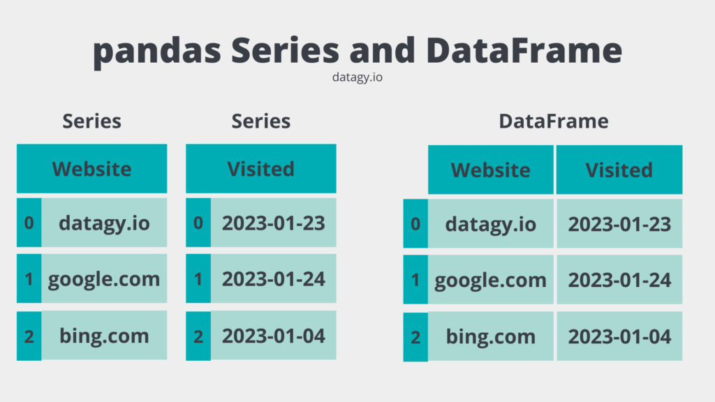
Because the DataFrame is a container for the Series, they can also share a similar language for accessing, manipulating, and working with the data. Similarly, by providing two data structures, pandas makes it much easier to work with two-dimensional data.

We’ll focus more on the Pandas DataFrame in this guide. This is because it’s a much more common data structure you’ll encounter in your day-to-day work. Now, let’s dive into how we can create a Pandas DataFrame from scratch.

Creating Pandas DataFrames from Scratch

To create a Pandas DataFrame, you can pass data directly into the pd.DataFrame() constructor. This allows you to pass in different types of Python data structures, such as lists, dictionaries, or tuples.

Loading a List of Tuples into a pandas DataFrame

Pandas can infer a lot about the data that you pass in, meaning that you have less work to do. Imagine that you’re working with data extracted from a database, where the data are stored as lists of tuples. For example, you might find data that looks like this:

# Sample List of Tuples Dataset
data = [
    ('Nik', 34, '2022-12-12'),
    ('Katie', 33, '2022-12-01'),
    ('Evan', 35, '2022-02-02'),
    ('Kyra', 34, '2022-04-14')
]

We can pass this dataset directly into the constructor and pandas will figure out how to split the columns into a meaningful, tabular dataset. Let’s see what this looks like:

# Loading a List of Tuples into a Pandas DataFrame
import pandas as pd
data = [
    ('Nik', 34, '2022-12-12'),
    ('Katie', 33, '2022-12-01'),
    ('Evan', 35, '2022-02-02'),
    ('Kyra', 34, '2022-04-14')
]

df = pd.DataFrame(data)
print(df)

# Returns:
#        0   1           2
# 0    Nik  34  2022-12-12
# 1  Katie  33  2022-12-01
# 2   Evan  35  2022-02-02
# 3   Kyra  34  2022-04-14

We can see that pandas was able to parse out the individual rows and columns of the dataset. Each tuple in the list is parsed as a single row, while each tuple scalar is identified as a column in the dataset.

Note that pandas didn’t assign any column names. This makes sense, since we didn’t ask it to! Instead, it used numbering from 0 through 2. Let’s see how we can add meaningful columns to the DataFrame by using the columns= parameter in the constructor.

# Adding Columns Names to Our DataFrame
import pandas as pd
data = [
    ('Nik', 34, '2022-12-12'),
    ('Katie', 33, '2022-12-01'),
    ('Evan', 35, '2022-02-02'),
    ('Kyra', 34, '2022-04-14')
]

df = pd.DataFrame(data, columns=['Name', 'Age', 'Date Joined'])
print(df)

# Returns:
#     Name  Age Date Joined
# 0    Nik   34  2022-12-12
# 1  Katie   33  2022-12-01
# 2   Evan   35  2022-02-02
# 3   Kyra   34  2022-04-14

We can see from the DataFrame above that we were able to pass in a list of column headers by using the columns= parameter. pandas makes it simple and intuitive to create tabular data structures that are easily represented in a familiar format.

Loading a List of Dictionaries into a pandas DataFrame

In other cases, you might get data in a list of dictionaries. Think of loading JSON data from a web API – in many cases, this data comes in the format of a list of dictionaries. Take a look at what this looks like below:

# A List of Dictionaries
[{'Name': 'Nik', 'Age': 34, 'Date Joined': '2022-12-12'},
 {'Name': 'Katie', 'Age': 33, 'Date Joined': '2022-12-01'},
 {'Name': 'Evan', 'Age': 35, 'Date Joined': '2022-02-02'},
 {'Name': 'Kyra', 'Age': 34, 'Date Joined': '2022-04-14'}]

We can load this dataset, again, by passing it directly into the pd.DataFrame() constructor, as shown below:

# Loading a List of Dictionaries into a Pandas DataFrame
import pandas as pd
data = [
    {'Name': 'Nik', 'Age': 34, 'Date Joined': '2022-12-12'},
    {'Name': 'Katie', 'Age': 33, 'Date Joined': '2022-12-01'},
    {'Name': 'Evan', 'Age': 35, 'Date Joined': '2022-02-02'},
    {'Name': 'Kyra', 'Age': 34, 'Date Joined': '2022-04-14'}
]

df = pd.DataFrame(data)
print(df)

# Returns:
#     Name  Age Date Joined
# 0    Nik   34  2022-12-12
# 1  Katie   33  2022-12-01
# 2   Evan   35  2022-02-02
# 3   Kyra   34  2022-04-14

You can see in the code block above that we didn’t need to pass in column names. pandas knows to use the dictionary keys in order to parse out column headers.

Now that we’ve learned how to create pandas DataFrames, let’s take a look at how we can read premade datasets into them.

Reading Data into Pandas DataFrames

pandas offers a lot of functionality for reading different data types into DataFrames. For example, you can read data from Excel files, text files (like CSV), SQL databases, web APIs stored in JSON data, and even directly from webpages!

Let’s take a look at how we can load a CSV file. pandas provides the option of loading the dataset either as a file stored on your computer or as a file it can download from a webpage. Take a look at the dataset here. You can either download it or work with it as the webpage (though, you’ll need an active internet connection, of course).

pandas offers a number of custom functions for loading in different types of datasets:

• The pandas .read_csv() function is used for reading CSV files into a pandas DataFrame
• The pandas .read_excel() function is used for reading Excel files into a pandas DataFrame
• The pandas .read_html() function is used for reading HTML tables into a pandas DataFrame
• The pandas .read_parquet() function is used for reading parquet files into a pandas DataFrame
• and many more…

Let’s see how we can use the pandas read_csv() function to read the CSV file we just described.

# Loading a CSV File into a Pandas DataFrame
import pandas as pd
df = pd.read_csv('https://raw.githubusercontent.com/datagy/data/main/data.csv')
print(df)

# Returns:
#            Date Region                 Type  Units   Sales
# 0    2020-07-11   East  Children's Clothing   18.0   306.0
# 1    2020-09-23  North  Children's Clothing   14.0   448.0
# 2    2020-04-02  South     Women's Clothing   17.0   425.0
# 3    2020-02-28   East  Children's Clothing   26.0   832.0
# 4    2020-03-19   West     Women's Clothing    3.0    33.0
# ..          ...    ...                  ...    ...     ...
# 995  2020-02-11   East  Children's Clothing   35.0   735.0
# 996  2020-12-25  North       Men's Clothing    NaN  1155.0
# 997  2020-08-31  South       Men's Clothing   13.0   208.0
# 998  2020-08-23  South     Women's Clothing   17.0   493.0
# 999  2020-08-17  North     Women's Clothing   25.0   300.0

# [1000 rows x 5 columns]

Let’s break down what we did in the code block above:

1. We imported the pandas library using the conventional alias pd
2. We then created a new variable df, which is the convention used to create a pandas DataFrame. For this variable, we used the pd.read_csv() function, which requires only a a string to the path containing the file. pandas can read files hosted remotely or on your local machine. In this case, we’re using a dataset hosted remotely.
3. Finally, we printed the DataFrame using the Python print() function. Pandas printed out the first five records and the last five records. However, it also provided information on the actual size of the dataset, indicating that it includes 1000 rows and 5 columns.

Tip! Pandas makes it easy to count the number of rows in a DataFrame, as well as counting the number of columns in a DataFrame using special methods.

Python and pandas will truncate the DataFrame based on the size of your terminal and the size of the DataFrame. You can control this a lot further by forcing pandas to show all rows and columns. However, we can also ask pandas to show specific data using additional methods. Let’s dive into this next.

Viewing Data in Pandas

pandas provides a lot of functionality in order to see the data that’s stored within a DataFrame. So far, you have learned that you can print a DataFrame, simply by passing it into the Python print() function. Depending on how much data is stored in your DataFrame, the output will be truncated.

We can use different DataFrame method to learn more about our data. For example:

• the .head(n) method returns the first n rows of a DataFrame (and defaults to five rows),
• the .last(n) method returns the last n rows of a DataFrame (and defaults to five rows),
• accessors like .iloc[x:y, :] will return rows x through y-1,
• and many more

Let’s see how we can dive into some of the data by using these methods. First, we’ll print the first five rows of the DataFrame:

# Printing the First Five Rows of a DataFrame
import pandas as pd
df = pd.read_csv('https://raw.githubusercontent.com/datagy/data/main/data.csv')
print(df.head())

# Returns:
#            Date Region                 Type  Units   Sales
# 0    2020-07-11   East  Children's Clothing   18.0   306.0
# 1    2020-09-23  North  Children's Clothing   14.0   448.0
# 2    2020-04-02  South     Women's Clothing   17.0   425.0
# 3    2020-02-28   East  Children's Clothing   26.0   832.0
# 4    2020-03-19   West     Women's Clothing    3.0    33.0

Notice in the code block above, that we didn’t need to pass in a number into the .head() method. By default, pandas will use a value of 5. This allows you to easily print out the first five rows of the DataFrame.

Similarly, we can print out the last n records of the DataFrame. The .tail() method defaults to five, similar to the .head() method. Let’s see how we can use the method specify wanting to print the last three records:

# Printing the Last n Rows of a DataFrame
import pandas as pd
df = pd.read_csv('https://raw.githubusercontent.com/datagy/data/main/data.csv')
print(df.tail(3))

# Returns:
#            Date Region              Type  Units  Sales
# 997  2020-08-31  South    Men's Clothing   13.0  208.0
# 998  2020-08-23  South  Women's Clothing   17.0  493.0
# 999  2020-08-17  North  Women's Clothing   25.0  300.0

We can see how simple that was! We’ll save using the .iloc accessor for a later section, since it goes beyond just returning rows. For now, let’s dive a little bit into what actually makes up a pandas DataFrame.

What Makes Up a Pandas DataFrame

Before we dive further into working with pandas DataFrames, let’s explore what makes up a DataFrame to begin with. The pandas library documentation itself defines a DataFrame as:

Two-dimensional, size-mutable, potentially heterogeneous tabular data.

pandas DataFrame documentation (link)

Oof. That’s a mouthful. Let’s break this down, step by step:

• two-dimensional means it has both rows and columns,
• size-mutable means that the size and shape can change as the DataFrame grows or its shape is modified, and
• potentially heterogeneous means that the data type can be different across columns

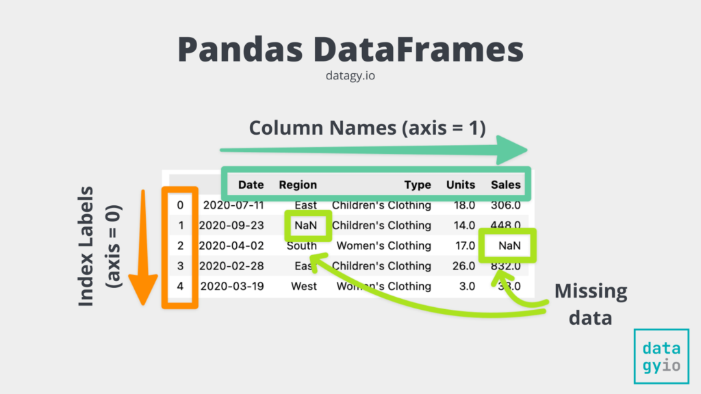
Now that we know what a DataFrame can be, let’s take a look at what makes it up. Take a look at the image below, which represents a pretty-printed version of our DataFrame:

Let’s take a look at the individual components of a pandas DataFrame:

• The index represents the “row” labels of a dataset. In pandas, the index is also represented as the 0^th axis. You can see how the index of our DataFrame above are bolded numbers from 0 through the end. In this case the index labels are arbitrary, but can also represent unique, intelligible values.
• The columns are represented by the 1st axis of the DataFrame and are each made up of individual pandas Series objects. Each column can have a unique data type, though joined together the DataFrame can be heterogeneous.
• The actual data can be of different data types, including dates. The data can also contain missing data, as represented by the NaN (not a number) values.

Now that you have a good understanding of how DataFrames are built up, let’s dive back into selecting data.

Selecting Columns and Rows in Pandas

Pandas provides a number of simple ways to select data, either as rows, columns, or cross-sections. Let’s take a look at some high-level options first. Imagine that we’re working with the same DataFrame we’ve used so far that looks like this:

# Showing Our DataFrame
import pandas as pd
df = pd.read_csv('https://raw.githubusercontent.com/datagy/data/main/data.csv')
print(df.head())

# Returns:
#          Date Region                 Type  Units  Sales
# 0  2020-07-11   East  Children's Clothing   18.0  306.0
# 1  2020-09-23  North  Children's Clothing   14.0  448.0
# 2  2020-04-02  South     Women's Clothing   17.0  425.0
# 3  2020-02-28   East  Children's Clothing   26.0  832.0
# 4  2020-03-19   West     Women's Clothing    3.0   33.0

The table below breaks down the different options we have to select data in our Pandas DataFrame:

1. df.iloc[] is used to select values based on their integer location,
2. df.loc[] is used to select values based on their labels,
3. df[col_name] is used to select an entire column (or a list of columns) of data
4. df[n] is used to return a single row (or a range of rows)

Using .iloc and .loc to Select Data in Pandas

Let’s see how we can use the .iloc[] accessor to select some rows and data from our pandas DataFrame:

# Using .iloc to Select Data
import pandas as pd
df = pd.read_csv('https://raw.githubusercontent.com/datagy/data/main/data.csv')
print(df.iloc[0,0])

# Returns: 2020-07-11

pandas, like Python, is 0-based indexed. This means that on each of our axes, the data starts at index 0. Because of this, returning df.iloc[0,0] will return the value from the first row in the first column.

Similarly, we can use the .loc[] accessor to access values based on their labels. Because our index uses arbitrary labels, we’ll specify the selection using the row number, as shown below:

# Using .loc to Select Data
import pandas as pd
df = pd.read_csv('https://raw.githubusercontent.com/datagy/data/main/data.csv')
print(df.loc[1,'Units'])

# Returns: 14.0

In the code block above, we asked Pandas to select the data from the row of index 1 (our second row) and from the 'Units' column. This method can make a lot more sense when our index labels are intelligible, such as using dates or specific people.

We can also select range of data using slicing. Both the .iloc and .loc methods allow you to pass in slices of data, such as df.iloc[:4, :] which would return rows 0-3 and all columns.

Selecting Entire Rows and Columns

You can also select entire rows and columns of data. Pandas will accept numeric values and ranges to select entire rows of data. If, for example, you wanted to select rows with positions 3 through 10, you could use the following code:

# Selecting a Range of Rows in a Pandas DataFrame
import pandas as pd
df = pd.read_csv('https://raw.githubusercontent.com/datagy/data/main/data.csv')
print(df[3:10])

# Returns: 
#           Date Region                 Type  Units  Sales
# 3   2020-02-28   East  Children's Clothing   26.0  832.0
# 4   2020-03-19   West     Women's Clothing    3.0   33.0
# 5   2020-02-05  North     Women's Clothing   33.0  627.0
# 6   2020-01-24  South     Women's Clothing   12.0  396.0
# 7   2020-03-25   East     Women's Clothing   29.0  609.0
# 8   2020-01-03  North  Children's Clothing   18.0  486.0
# 9   2020-11-03   East  Children's Clothing   34.0  374.0
# 10  2020-04-16  South     Women's Clothing   16.0  352.0

We can see that this includes data up to row label 10, but not including. It’s worth noting, here, that we were able to omit the .iloc[] accessor here. pandas is able to infer that we want to select the rows.

Similarly, you can select an entire column by simply indexing its name. This returns a Pandas Series, as shown below:

# Selecting a Column from a Pandas DataFrame
import pandas as pd
df = pd.read_csv('https://raw.githubusercontent.com/datagy/data/main/data.csv')
print(df['Date'])

# Returns: 
# 0      2020-07-11
# 1      2020-09-23
# 2      2020-04-02
# 3      2020-02-28
# 4      2020-03-19
#           ...    
# 995    2020-02-11
# 996    2020-12-25
# 997    2020-08-31
# 998    2020-08-23
# 999    2020-08-17
# Name: Date, Length: 1000, dtype: object

You can also select a number of different columns. To do this, pass a list into the indexing. Let’s select the 'Date' and 'Type' column:

# Selecting Columns from a Pandas DataFrame
import pandas as pd
df = pd.read_csv('https://raw.githubusercontent.com/datagy/data/main/data.csv')
print(df[['Date', 'Type']])

# Returns: 
#            Date                 Type
# 0    2020-07-11  Children's Clothing
# 1    2020-09-23  Children's Clothing
# 2    2020-04-02     Women's Clothing
# 3    2020-02-28  Children's Clothing
# 4    2020-03-19     Women's Clothing
# ..          ...                  ...
# 995  2020-02-11  Children's Clothing
# 996  2020-12-25       Men's Clothing
# 997  2020-08-31       Men's Clothing
# 998  2020-08-23     Women's Clothing
# 999  2020-08-17     Women's Clothing

# [1000 rows x 2 columns]

Note that we were able to select the columns without them needing to be beside one another! Doing this returns a pandas DataFrame.

To learn more about selecting and finding data, check out the resources below:

• How to Index, Select and Assign Data in Pandas
• How to Select Columns in Pandas
• How to Shuffle Pandas Dataframe Rows in Python
• How to Sample Data in a Pandas DataFrame
• How to Split a Pandas DataFrame
• Reorder Pandas Columns: Pandas Reindex and Pandas insert
• Pandas: How to Drop a Dataframe Index Column
• Pandas Reset Index: How to Reset a Pandas Index
• Pandas Rename Index: How to Rename a Pandas Dataframe Index

Filtering Data in Pandas DataFrames

Pandas makes it simple to filter the data in your DataFrame. In fact, it provides many different ways in which you can filter your dataset. In this section, we’ll explore a few of these different method and provide you with further resources to take your skills to the next level.

Let’s see what happens when we apply a logical operator to a pandas DataFrame column:

# Applying a Boolean Operator to a Pandas Column
import pandas as pd
df = pd.read_csv('https://raw.githubusercontent.com/datagy/data/main/data.csv', parse_dates=['Date'])
print(df['Units'] > 30)

# Returns:
# 0      False
# 1      False
# 2      False
# 3      False
# 4      False
#        ...  
# 995     True
# 996    False
# 997    False
# 998    False
# 999    False
# Name: Units, Length: 1000, dtype: bool

When we apply a boolean operator to a pandas DataFrame column, this returns a boolean Series of data. On the surface, this may not look very helpful. However, we can index our DataFrame with this Series to filter our data! Let’s see what this looks like:

# Filtering a Pandas DataFrame with Logical Operators
import pandas as pd
df = pd.read_csv('https://raw.githubusercontent.com/datagy/data/main/data.csv', parse_dates=['Date'])
print(df[df['Units'] > 30])

# Returns:
#           Date Region                 Type  Units   Sales
# 5   2020-02-05  North     Women's Clothing   33.0   627.0
# 9   2020-11-03   East  Children's Clothing   34.0   374.0
# 16  2020-06-12   East     Women's Clothing   35.0  1050.0
# 18  2020-06-16  North     Women's Clothing   34.0   884.0
# 20  2020-09-14  North  Children's Clothing   35.0   630.0
# ..         ...    ...                  ...    ...     ...
# 973 2020-10-04   East       Men's Clothing   35.0   350.0
# 977 2020-10-20   East       Men's Clothing   32.0   928.0
# 985 2020-02-08   West       Men's Clothing   32.0   928.0
# 987 2020-04-23  South     Women's Clothing   34.0   680.0
# 995 2020-02-11   East  Children's Clothing   35.0   735.0

# [146 rows x 5 columns]

We can see that by indexing our DataFrame using the boolean condition that pandas filters our DataFrame.

pandas also provides a helpful method to filter a DataFrame. This can be done using the pandas .query() method, which allows you to use plain-language style queries to filter your DataFrame.

Let’s dive into exploring the Pandas query() function to better understand the parameters and default arguments that the function provides.

# Understanding the Pandas query() Function
import pandas as pd
DataFrame.query(expr, inplace=False, **kwargs)

We can see that the Pandas query() function has two parameters:

1. expr= represents the expression to use to filter the DataFrame
2. inplace= instructs Pandas to filter the DataFrame in place and defaults to False

The Pandas .query() method lets you pass in a string that represents a filter expression. The syntax can feel a little awkward at first but if you’re familiar with SQL, the format will feel very natural. Let’s take a look at an example where we filter the DataFrame to show only rows where Units are less than 4.

import pandas as pd
df = pd.read_excel(
    'https://github.com/datagy/mediumdata/raw/master/sample_pivot.xlsx',
    parse_dates=['Date']
)

filtered = df.query('Units < 4')
print(filtered.head())

# Returns:
#           Date Region                 Type  Units  Sales
# 4   2020-03-19   West     Women's Clothing    3.0     33
# 28  2020-01-19   East       Men's Clothing    3.0     63
# 96  2020-11-13   East  Children's Clothing    3.0     72
# 118 2020-12-28   East  Children's Clothing    3.0     78
# 134 2020-09-04  North  Children's Clothing    3.0    184

We can see that by passing in a string that represents the expression, in this case 'Units < 4'. In this example, we filtered a numeric column.

The Pandas query method can also be used to filter with multiple conditions. This allows us to specify conditions using the logical and or or operators. By using multiple conditions, we can write powerful statements that filter based on single or multiple columns.

Let’s see how we can use the method to filter data based on the Region and Units column.

import pandas as pd
df = pd.read_excel(
    'https://github.com/datagy/mediumdata/raw/master/sample_pivot.xlsx',
    parse_dates=['Date']
)

filtered = df.query('Region == "West" and Units < 4')
print(filtered.head())

# Returns:
#           Date Region                 Type  Units  Sales
# 4   2020-03-19   West     Women's Clothing    3.0     33
# 135 2020-01-07   West     Women's Clothing    3.0    350
# 355 2020-06-12   West  Children's Clothing    3.0    567
# 558 2020-10-06   West       Men's Clothing    3.0    462
# 686 2020-02-18   West       Men's Clothing    3.0    918

In the example above, we pass in two conditions: one based on a numeric column and another based on a string column. We use the and operator to make sure that both conditions are met.

To learn more about how to filter DataFrames in pandas, check out the resources below:

• How to Filter a Pandas DataFrame
• How to Use Pandas Query to Filter a DataFrame
• How to Use Pandas Isin to Filter a Dataframe like SQL IN and NOT IN

Writing Pandas DataFrames to Files

So far, we’ve explored how to load data and view the data. Another thing you’re probably keen to learn is how to save the DataFrames that you’re working. Thankfully, pandas supports many different files types to save to. Many of these methods are logically named: for example, .to_excel() is used to save a DataFrame to an Excel file.

Let’s see how we can use the pandas .to_csv() method to save a DataFrame to a CSV file. The method provides a lot of flexibility in terms of how you save the data. For example, you can choose to include or exclude the DataFrames index when saving the file.

# Saving a Pandas DataFrame to a CSV File
import pandas as pd
df = pd.read_csv('https://raw.githubusercontent.com/datagy/data/main/data.csv')
df.to_csv('file.csv', sep=';', index=False)

In the example above, we used the .to_csv() method to save a pandas DataFrame to a CSV file. Note that we used three parameters:

1. 'file.csv' is the file name to which we want to save the file to,
2. 'sep=';' indicates that we want the file to be separated by semi-colons, and
3. index=False indicates that we want to save the file without the index included.

Not including an index is often done when the index is arbitrary. In our case, the index only represents the row number. Because of this, it makes sense to exclude it from our resulting file.

In order to save pandas DataFrames to different data formats, you can use the methods outlined below:

• pandas .to_excel() method is used to save pandas DataFrames to Excel files
• pandas .to_csv() method is used to save pandas DataFrames to CSV files
• pandas .values.tolist() method is used to save pandas DataFrames to Python lists
• pandas .to_dict() method is used to save pandas DataFrames to Python dictionaries
• pandas .to_json() method is used to save pandas DataFrames to JSON files
• pandas .to_pickle() method is used to save pandas DataFrames to pickle files

Let’s now dive into how to use Pandas to describe our dataset.

Describing Data with Pandas

Pandas provides many different ways in which you can analyze your data. However, it can often be very helpful to first get a sense of what the data in your DataFrame is. For this, you can use two main DataFrame methods:

1. .info() provides information about the DataFrame itself, and
2. .describe() provides information about the data in the DataFrame

Let’s take a look at the .info() method first. The method can be applied directly to the DataFrame and will return information about the DataFrame, such as its size, columns, and more. Let’s see what happens when we print the result from the df.info() method.

# Using the .info() Method to Display Information
import pandas as pd
df = pd.read_csv('https://raw.githubusercontent.com/datagy/data/main/data.csv')
print(df.info())

# Returns:
# <class 'pandas.core.frame.DataFrame'>
# RangeIndex: 1000 entries, 0 to 999
# Data columns (total 5 columns):
#  #   Column  Non-Null Count  Dtype  
# ---  ------  --------------  -----  
#  0   Date    1000 non-null   object 
#  1   Region  1000 non-null   object 
#  2   Type    1000 non-null   object 
#  3   Units   911 non-null    float64
#  4   Sales   1000 non-null   float64
# dtypes: float64(2), object(3)
# memory usage: 39.2+ KB

In the code block above, we can see that the method returns a lot of useful information. For example, we can see that the index is a RangeIndex, meaning it contains the values from 0 through 999.

Similarly, we can see that the DataFrame contains five columns. We can also see their data types and how many non-null values are in each column. Finally, we can see the memory usage of the DataFrame.

Let’s now take a look at the .descibe() method, which allows us to describe the data that’s within the DataFrame itself. This allows you to see information about the numeric columns by providing high-level statistics.

import pandas as pd
df = pd.read_csv('https://raw.githubusercontent.com/datagy/data/main/data.csv')
print(df.describe())

# Returns:
#             Units        Sales
# count  911.000000  1000.000000
# mean    19.638858   427.254000
# std      9.471309   253.441362
# min      3.000000    33.000000
# 25%     12.000000   224.000000
# 50%     20.000000   380.000000
# 75%     28.000000   575.000000
# max     35.000000  1155.000000

We can see that the method returned useful information, such as the number of data points, the mean values, standard deviation and other statistics.

To learn more about the pandas .describe() method, this guide provides you with everything you need to know about the describe method.

Analyzing Data with Pandas

Being an analytics library, pandas provides a ton of different options to analyze your data. In fact, there are built-in methods for really anything that you may want to do. If there aren’t, it’s simple and intuitive to build your own methods.

Let’s take a look at some simple descriptive statistics first. Many of the methods provide easy to understand names. For example, to calculate the mean, you can use the .mean() method. This is where the Pandas API becomes even more interesting. Many of the methods are available for both a pandas Series as well as for DataFrames. pandas will change the resulting output, depending on what object type the method is applied to. Let’s see how we can calculate the mean for a pandas column first:

# Calculating the Mean of a Pandas Column
import pandas as pd
df = pd.read_csv('https://raw.githubusercontent.com/datagy/data/main/data.csv')
print(df['Sales'].mean())

# Returns: 427.254

We can see that when we apply the method to a single pandas Series column, that the method returns a single value scalar. In this case, that value is 427.254.

Similarly, we can apply the method to an entire DataFrame. Let’s see how this changes the output:

# Calculating the Mean for a DataFrame
import pandas as pd
df = pd.read_csv('https://raw.githubusercontent.com/datagy/data/main/data.csv')
print(df.mean(numeric_only=True))

# Returns: 
# Units     19.638858
# Sales    427.254000
# dtype: float64

When we apply the .mean() method to an entire DataFrame, we need to use the numeric=True argument, specifying that we want to only apply the method to the numeric columns of the DataFrame. By doing this, pandas will return a Series of data. This means that we can actually access the individual means by indexing them.

pandas provides many other methods for calculating statistics. You can learn more about them by checking out the resources below. You can even use custom functions and work with them to transform pandas columns using the .map() and .apply().methods. Similarly, you can easily create conditional columns in pandas in a variety of ways.

• How to Sum Columns in Pandas
• How to Calculate Quantiles in Pandas
• How to Calculate a Weighted Average in Pandas
• How to Calculate a Rolling Average in Pandas
• How to Calculate the Standard Deviation in Pandas
• How to Calculate the Median Absolute Deviation in Pandas
• How to Calculate a Z-Score in Pandas
• How to Normalize a Pandas Column or Dataframe
• How to Calculate the Variance in Pandas
• How to Calculate the Difference Between Pandas Rows
• How to Calculate Crosstabs in Pandas

Sorting Data and Working with Duplicate Data

In this section, we’ll dive into how to work with pandas DataFrames to sort data and to work with duplicate data. As is to be expected, pandas offers significant functionality for allowing you to sort data and work with duplicate data.

How to Sort Data in a Pandas DataFrame

Let’s see how we can use the pandas .sort_values() method to sort data in our DataFrame. The method accepts a number of parameters, but let’s focus on some of the most important ones:

• by= allows you to pass in a single column label or a list of column labels to sort by
• ascending= accepts a boolean value to indicate if values should be sorted in ascending or descending order

Let’s see how we can sort by the 'Sales' column of our pandas DataFrame:

# Sorting Data in a Pandas DataFrame
import pandas as pd
df = pd.read_csv('https://raw.githubusercontent.com/datagy/data/main/data.csv')
df = df.sort_values(by='Sales', ascending=False)
print(df.head()

#            Date Region                 Type  Units   Sales
# 996  2020-12-25  North       Men's Clothing    NaN  1155.0
# 309  2020-09-11  North     Women's Clothing    5.0  1122.0
# 745  2020-12-09   East  Children's Clothing   23.0  1122.0
# 222  2020-05-28  South     Women's Clothing   13.0  1122.0
# 680  2020-07-03  North     Women's Clothing    4.0  1089.0

We can see from the code block above that the DataFrame has now been sorted. If you’re keen-eyed, you’ll notice as well that we reassigned the DataFrame to itself.

Methods applied to DataFrames don’t actually modify the DataFrame itself. We can force this behavior in many methods by passing in the inplace=True parameter. In many cases, however, you’ll see pandas users reassigning the DataFrame to itself.

How to Work with Duplicate Data in a Pandas DataFrame

pandas provides exceptional flexibility when working with duplicate data, including being able to identify, find, and remove duplicate fields. The pandas library acknowledges that data can be identified to be duplicate if all columns are equal, if some columns are equal, or if any columns are equal.

This allows you to have significant flexibility in terms of finding and dropping duplicate records. Let’s first take a look at finding duplicate records in a pandas DataFrame. This can be done by using the .duplicated() method, which returns a boolean array:

# Finding Duplicate Records in a Pandas DataFrame
import pandas as pd
df = pd.read_csv('https://raw.githubusercontent.com/datagy/data/main/data.csv')
print(df.duplicated().head())

# 0      False
# 1      False
# 2      False
# 3      False
# 4      False

In this case, we printed out the first five records of the resulting Series object. The Series contains boolean indications of whether or not a record at a specific index is a duplicate record or not.

By default, pandas will check if all values in the record are duplicated. We can check if there are any duplicate records by calculating the sum of this Series. Because True values are counted as 1 and False values are counted as 0, we can get a sense of the number of duplicate records this way:

# Counting Duplicate Records in a Pandas DataFrame
import pandas as pd
df = pd.read_csv('https://raw.githubusercontent.com/datagy/data/main/data.csv')
print(df.duplicated().sum())

# Returns: 0

In this case, we can see that our DataFrame has zero duplicate records. By what about records that are duplicate across only a subset of columns? For this, we can use the subset= parameter, which accepts either a column label or a list of labels as input.

Let’s count how many duplicate records there are across the ['Type', 'Region'] columns:

# Counting Duplicate Records in a Pandas DataFrame
import pandas as pd
df = pd.read_csv('https://raw.githubusercontent.com/datagy/data/main/data.csv')
print(df.duplicated(subset=['Type', 'Region']).sum())

# Returns: 998

We can see that in this case we have 998 duplicate records.

Now that we know how to count duplicate records, let’s take a look at how we remove duplicate records in a pandas DataFrame. In order to do this, we can use the aptly-named .drop_duplicates() method.

Similar to the .duplicated() method, the .drop_duplicates() method allows you select only a subset of columns. However, it also allows you to use the following additional parameters:

• subset= which allows you to specify the columns to consider,
• keep= identifies which record to keep,
• inplace= will drop the records in place if the argument is set to True, and
• ignore_index= will reset the index following dropping values

Let’s see how we can use the method to drop duplicates across the ['Type', 'Region'] columns:

# Dropping Duplicates in Pandas
# Dropping Duplicate Records in a Pandas DataFrame
import pandas as pd
df = pd.read_csv('https://raw.githubusercontent.com/datagy/data/main/data.csv')
df = df.drop_duplicates(subset=['Type', 'Region'])
print(df)

# Returns:
#           Date Region                 Type  Units  Sales
# 0   2020-07-11   East  Children's Clothing   18.0  306.0
# 1   2020-09-23  North  Children's Clothing   14.0  448.0
# 2   2020-04-02  South     Women's Clothing   17.0  425.0
# 4   2020-03-19   West     Women's Clothing    3.0   33.0
# 5   2020-02-05  North     Women's Clothing   33.0  627.0
# 7   2020-03-25   East     Women's Clothing   29.0  609.0
# 11  2020-08-09  North       Men's Clothing    NaN  270.0
# 12  2020-05-01   East       Men's Clothing   10.0  140.0
# 15  2020-11-26   West       Men's Clothing   27.0  864.0
# 30  2020-07-13   West  Children's Clothing   30.0  450.0
# 42  2020-03-17  South  Children's Clothing   33.0  924.0
# 57  2020-07-23  South       Men's Clothing   27.0  351.0

In the example above, our DataFrame has been reduced to only twelve records! You may be wondering how pandas chose which records to keep and which records to drop. By default, the method will keep the first item for which records are duplicated.

Knowing this, gives you significant flexibility of how to identify records to be dropped. By combining what you learned about sorting values, you can make sure you’re keeping the most appropriate records when dropping records in pandas.

Let’s now dive into another important topic: working with missing data.

Dealing with Missing Data in Pandas

When working with missing data, you generally have two different options:

1. Drop the records that contain missing data, or
2. Fill the missing data with a certain value.

You may remember from earlier, when we used the .info() method, that we were able to see how many non-missing records exist in each column. Let’s take a look at this again:

# Using the .info() Method to Display Information
import pandas as pd
df = pd.read_csv('https://raw.githubusercontent.com/datagy/data/main/data.csv')
print(df.info())

# Returns:
# <class 'pandas.core.frame.DataFrame'>
# RangeIndex: 1000 entries, 0 to 999
# Data columns (total 5 columns):
#  #   Column  Non-Null Count  Dtype  
# ---  ------  --------------  -----  
#  0   Date    1000 non-null   object 
#  1   Region  1000 non-null   object 
#  2   Type    1000 non-null   object 
#  3   Units   911 non-null    float64
#  4   Sales   1000 non-null   float64
# dtypes: float64(2), object(3)
# memory usage: 39.2+ KB

By doing some additional math, we can see that the Units column has 89 missing data. In this case, this was simple to calculate. However, working with different datasets, this can actually get a little complicated (not to mention annoying).

We can actually simplify this process using the pandas .isna() method and adding up the boolean DataFrame it returns using the .sum() method. Let’s see what this looks like:

# Counting Missing Records in a Pandas DataFrame
import pandas as pd
df = pd.read_csv('https://raw.githubusercontent.com/datagy/data/main/data.csv')
print(df.isna().sum())

# Returns:
# Date       0
# Region     0
# Type       0
# Units     89
# Sales      0
# dtype: int64

Now that we know how to count missing records, let’s dive into working with these missing values. We’ll explore both dropping and filling missing data, but let’s kick things off by taking a look at how to drop missing data from a dataset in pandas.

How to Drop Missing Data in Pandas

The Pandas .dropna() method is an essential method for a data analyst or data scientist of any level. Because cleaning data is an essential preprocessing step, knowing how to work with missing data will make you a stronger programmer.

Before diving into how to use the method, let’s take a minute to understand how the Pandas .dropna() method works. We can do this by taking a look at the parameters and default arguments that method provides:

# Understanding the Pandas .dropna() Method
import pandas as pd
df = pd.DataFrame()

df.dropna(
   axis=0,
   how='any',
   thresh=None,
   subset=None,
   inplace=False
)

The Pandas dropna() method makes it very easy to drop all rows with missing data in them. By default, the Pandas dropna() will drop any row with any missing record in it. This is because the how= parameter is set to 'any' and the axis= parameter is set to 0.

Let’s see what happens when we drop missing data from our DataFrame:

# Dropping Duplicate Records in a Pandas DataFrame
import pandas as pd
df = pd.read_csv('https://raw.githubusercontent.com/datagy/data/main/data.csv')
df = df.dropna()
print(df.isna().sum())

# Returns:
# Date       0
# Region     0
# Type       0
# Units      0
# Sales      0
# dtype: int64

We can see that by applying the .dropna() method on the DataFrame dropped any record that contained any missing value. The pandas .dropna() method provides significant flexibility in how to drop records with missing data, such as ensuring that certain columns must be missing.

Now, let’s explore how to fill missing data in pandas.

How to Fill Missing Data in Pandas

The pandas .fillna() method is used to fill missing values with a certain value in a DataFrame. The method lets you pass in a value to fill missing records with. Let’s see how we can fill the missing values in the 'Units' column with the value 0.

# Filling Missing Data in a Column
import pandas as pd
df = pd.read_csv('https://raw.githubusercontent.com/datagy/data/main/data.csv')
df = df.sort_values(by='Units')
df['Units'] = df['Units'].fillna(0)
print(df)

# Returns:
#            Date Region              Type  Units   Sales
# 141  2020-02-12   East  Women's Clothing    3.0   330.0
# 28   2020-01-19   East    Men's Clothing    3.0    63.0
# 686  2020-02-18   West    Men's Clothing    3.0   918.0
# 310  2020-02-25   East    Men's Clothing    3.0   330.0
# 684  2020-04-08   East    Men's Clothing    3.0   806.0
# ..          ...    ...               ...    ...     ...
# 927  2020-02-24  North    Men's Clothing    0.0   210.0
# 939  2020-02-26  North    Men's Clothing    0.0   300.0
# 945  2020-04-12  North    Men's Clothing    0.0   364.0
# 946  2020-01-30  North    Men's Clothing    0.0   285.0
# 996  2020-12-25  North    Men's Clothing    0.0  1155.0

# [1000 rows x 5 columns]

We can see in the example above that all our missing data was filled with the value 0. Note, we had sorted the DataFrame so that the missing data was at the end of the DataFrame. Similarly, you can instruct pandas to fill the missing data with another calculated value, such as the mean of the column. This can be done by passing in df['Units'].mean() into the .fillna() method.

The method provides significant more flexibility, such as back-filling or forward-filling missing data, which can be incredibly useful when working with time series data.

Pandas Pivot Tables and Reshaping Data

A pivot table is a table of statistics that helps summarize the data of a larger table by “pivoting” that data. Microsoft Excel popularized the pivot table, where they’re known as PivotTables. Pandas gives access to creating pivot tables in Python using the .pivot_table() function. The function has the following default parameters:

# The syntax of the .pivot_table() function
import pandas as pd
pd.pivot_table(
    data=,
    values=None, 
    index=None, 
    columns=None, 
    aggfunc='mean', 
    fill_value=None, 
    margins=False, 
    dropna=True, 
    margins_name='All', 
    observed=False,
    sort=True
) 

Let’s create your first Pandas pivot table. At a minimum, we have to pass in some form of a group key, either using the index= or columns= parameters. In the examples below, we’re using the Pandas function, rather than the DataFrame function. Because of this, we need to pass in the data= argument. If we applied the method to the DataFrame directly, this would be implied.

# Creating your first Pandas pivot table
pivot = pd.pivot_table(
    data=df,
    index='Region'
)
print(pivot)

# Returns:
#              Sales      Units
# Region                       
# East    408.182482  19.732360
# North   438.924051  19.202643
# South   432.956204  20.423358
# West    452.029412  19.29411

Let’s break down what happened here:

1. We created a new DataFrame called sales_by_region, which was created using the pd.pivot_table() function
2. We passed in our DataFrame, df, and set the index='region', meaning data would be grouped by the region column

Because all other parameters were left to their defaults, Pandas made the following assumption:

• Data should be aggregated by the average of each column (aggfunc='mean')
• The values should be any numeric columns

When we add columns to a Pandas pivot table, we add another dimension to the data. While the index= parameter splits the data vertically, the columns= parameter groups and splits the data horizontally. This allows us to create an easy-to-read table. Let’s see how we can use the columns= parameter to split the data by the Type column.

# Adding Columns to Our Pandas Pivot Table
pivot = pd.pivot_table(
    data=df,
    index='Region',
    columns='Type',
    values='Sales'
)

print(pivot)

# Returns:
# Type    Children's Clothing  Men's Clothing  Women's Clothing
# Region                                                       
# East             405.743363      423.647541        399.028409
# North            438.894118      449.157303        432.528169
# South            412.666667      475.435897        418.924528
# West             480.523810      465.292683        419.188679

We can see how easy it was to add a whole other dimension of data. This allows us to spot differences between groupings in a format that’s easy to read.

Pivot tables in pandas provide incredible versatility and flexibility of how you can analyze data in pandas. You can also reshape data using the melt function, which allows you to convert wide datasets into long datasets. Similarly, you can easily transpose pandas DataFrames using built-in and intuitive methods.

Grouping Data with Pandas Group By

The Pandas .groupby() method works in a very similar way to the SQL GROUP BY statement. In fact, it’s designed to mirror its SQL counterpart leverage its efficiencies and intuitiveness. Similar to the SQL GROUP BY statement, the Pandas method works by splitting our data, aggregating it in a given way (or ways), and re-combining the data in a meaningful way.

Because the .groupby() method works by first splitting the data, we can actually work with the groups directly. Similarly, because any aggregations are done following the splitting, we have full reign over how we aggregate the data. Pandas then handles how the data are combined in order to present a meaningful DataFrame.

The Pandas groupby method uses a process known as split, apply, and combine to provide useful aggregations or modifications to your DataFrame. This process works as just as its called:

1. Splitting the data into groups based on some criteria
2. Applying a function to each group independently
3. Combing the results into an appropriate data structure

In the section above, when you applied the .groupby() method and passed in a column, you already completed the first step! You were able to split the data into relevant groups, based on the criteria you passed in.

The reason for applying this method is to break a big data analysis problem into manageable parts. This allows you to perform operations on the individual parts and put them back together. While the apply and combine steps occur separately, Pandas abstracts this and makes it appear as though it was a single step.

Let’s take a look at how we can use the pandas .groupby() method to aggregate some data into different groups.

# Using the .groupby() Method to Aggregate Data
import pandas as pd
df = pd.read_csv('https://raw.githubusercontent.com/datagy/data/main/data.csv')
aggregate = df.groupby('Region')['Sales'].mean()
print(aggregate)

# Returns:
# Region
# East     408.182482
# North    438.924051
# South    432.956204
# West     452.029412
# Name: Sales, dtype: float64

We can see that the method can be used to group data in different ways. Once the data has been grouped, the data can be aggregated in different ways. In the example above, we used the .mean() method to aggregate the Sales data, broken out by the region.

To learn more about the pandas .groupby() method, check out this in-depth guide on aggregating data in pandas. Similarly, check out the resources below to find out different ways of using the method:

• Pandas Groupby and Aggregate for Multiple Columns
• Pandas: Count Unique Values in a GroupBy Object

Working with Dates in Pandas

In this section, we’ll dive into one of the truly incredible features of the pandas library: working with dates. One of the interesting things that we’ll explore here is that when we have loaded our data so far, it’s actually simply loaded just as strings. pandas represents the as the 'object' data type. We can change this behavior when we read our CSV file into a DataFrame. Let’s see what this looks like:

import pandas as pd
df = pd.read_csv('https://raw.githubusercontent.com/datagy/data/main/data.csv', parse_dates=['Date'])
print(df.info())

# Returns:
# <class 'pandas.core.frame.DataFrame'>
# RangeIndex: 1000 entries, 0 to 999
# Data columns (total 5 columns):
#  #   Column  Non-Null Count  Dtype         
# ---  ------  --------------  -----         
#  0   Date    1000 non-null   datetime64[ns]
#  1   Region  1000 non-null   object        
#  2   Type    1000 non-null   object        
#  3   Units   911 non-null    float64       
#  4   Sales   1000 non-null   float64       
# dtypes: datetime64[ns](1), float64(2), object(2)
# memory usage: 39.2+ KB
# None

In the example above, we added an additional parameter when loading our dataset: the parse_dates= parameter. This allows you to pass in a list of column labels to read in as dates. Now when we check out data types using the .info() method, our column is actually a datetime data type.

This now gives you access to an entire subset of date time attributes and functions. For example, we can access the month and year of a given date by using the .dt.month and .dt.year attributes of a datetime column. Let’s see what this looks like:

# Parsing Out Date Attributes in Pandas
import pandas as pd
df = pd.read_csv('https://raw.githubusercontent.com/datagy/data/main/data.csv', parse_dates=['Date'])
df['Year'] = df['Date'].dt.year
df['Month'] = df['Date'].dt.month
print(df.head())

# Returns:
#         Date Region                 Type  Units  Sales  Year  Month
# 0 2020-07-11   East  Children's Clothing   18.0  306.0  2020      7
# 1 2020-09-23  North  Children's Clothing   14.0  448.0  2020      9
# 2 2020-04-02  South     Women's Clothing   17.0  425.0  2020      4
# 3 2020-02-28   East  Children's Clothing   26.0  832.0  2020      2
# 4 2020-03-19   West     Women's Clothing    3.0   33.0  2020      3

Similarly, pandas is smart enough to use logical operators to filter dates! We can simply use greater than or less than operators to filter DataFrames based on their dates. Let’s see what this looks like:

# Filtering a Pandas DataFrame Based on Dates
import pandas as pd
df = pd.read_csv('https://raw.githubusercontent.com/datagy/data/main/data.csv', parse_dates=['Date'])
print(df[df['Date'] > '2020-12-01'].head())

# Returns:
#          Date Region                 Type  Units  Sales
# 32 2020-12-20   East     Women's Clothing   30.0  930.0
# 35 2020-12-17   West  Children's Clothing   25.0  575.0
# 38 2020-12-30  North  Children's Clothing   26.0  390.0
# 58 2020-12-25   East       Men's Clothing   13.0  403.0
# 81 2020-12-11  South     Women's Clothing   13.0  429.0

We can see that by passing in a logical operator into our filtering operation that pandas filtered our DataFrame to a specific range of dates.

To learn more about how to work with dates in pandas in and Python, check out the resources below;

• How to Use DateTime in Pandas and Python
• How to Use Pandas Datetime to Access Date Parts (Month, Year, etc.)
• How to Use Python to Convert a String to Date
• How to Use Python to Convert a Date to String
• How to Create Date Ranges with Pandas
• How to Get a Fiscal Year with Pandas
• Pandas to_datetime: Convert a Pandas String Column to Date Time
• How to Add Days to a Date Column in Pandas

Merging Data with Pandas

There are a number of different ways in which you may want to combine data. For example, you can combine datasets by concatenating them. This process involves combining datasets together by including the rows of one dataset underneath the rows of the other. This process will be referred to as concatenating or appending datasets.

There are a number of ways in which you can concatenate datasets. For example, you can require that all datasets have the same columns. On the other hand, you can choose to include any mismatched columns as well, thereby introducing the potential for including missing data.

Generally, the process of concatenating datasets will make your dataset longer, rather than wider. However, if you are comfortable with appending datasets with mismatched columns, the resulting dataset may also grow wider. Concatenating datasets focuses on merging based on columns, rather than based on records. This, is a generalization and is not always true!

You can also join datasets together, to make a larger one. This is what will be referred to as either joining or merging datasets in this tutorial. When you join a dataset with another, you are merging these sets based on a key (or keys).

Generally speaking, the process of merging datasets will focus on making the dataset wider, rather than longer. Depending on the overall between records, however, and the method of merging you choose, you may also introduce more rows. Merging datasets focuses on merging based on the records’ values, rather than based on column headers.

Appending Pandas DataFrames with .concat()

To follow along with this section, let’s load a few DataFrames to better understand the nuances of some how to combine Pandas DataFrames. We’ll load three different DataFrames with some overlap:

# Loading Sample Pandas DataFrames
import pandas as pd

df1 = pd.DataFrame.from_dict({'col1': [1, 2, 3], 'col2': ['a', 'b', 'c'], 'col3': ['a1', 'b2', 'c3']})
df2 = pd.DataFrame.from_dict({'col1': [4, 5, 6], 'col2': ['d', 'e', 'f'], 'col3': ['d4', 'e5', 'f6']})
df3 = pd.DataFrame.from_dict({'col1': [7, 8, 9], 'col2': ['g', 'h', 'i'], 'col4': ['g7', 'h2', 'i3']})

print('df1 looks like:')
print(df1)
print('\ndf2 looks like:')
print(df2)
print('\ndf3 looks like:')
print(df3)

# Returns:
# df1 looks like:
#    col1 col2 col3
# 0     1    a   a1
# 1     2    b   b2
# 2     3    c   c3

# df2 looks like:
#    col1 col2 col3
# 0     4    d   d4
# 1     5    e   e5
# 2     6    f   f6

# df3 looks like:
#    col1 col2 col4
# 0     7    g   g7
# 1     8    h   h2
# 2     9    i   i3

Let’s start by looking at the most straightforward example: concatenating two DataFrames with the same columns. The pandas concat() function can be used to append DataFrames with one another. It only requires you to pass in the objects you want to concatenate, you can simply pass in the list of objects. In this case, we can pass in [df1, df2]. Let’s see what this results in:

# Concatenating simple DataFrames
df_concat = pd.concat([df1, df2])
print(df_concat)

# Returns:
#    col1 col2 col3
# 0     1    a   a1
# 1     2    b   b2
# 2     3    c   c3
# 0     4    d   d4
# 1     5    e   e5
# 2     6    f   f6

Merging Pandas DataFrames Using .merge()

Pandas handles database-like joining operations with great flexibility. While, on the surface, the function works quite elegantly, there is a lot of flexibility under the hood. For example, you can complete many different merge types (such as inner, outer, left, and right) and merge on a single key or multiple keys.

In order to follow along with this tutorial, let’s load three simple DataFrames. Simply copy the code below to load these DataFrames to be able to better follow along with this section of the tutorial:

# Loading Sample DataFrames
books = pd.DataFrame.from_dict({
    'Author ID': [1,1,2,3],
    'Book ID': [1,2,1,1],
    'Name': ['Intro to Python', 'Python 201', 'Data Science', 'Machine Learning']})

authors = pd.DataFrame.from_dict({
    'Author ID': [1,2,3,4],
    'Name': ['Nik', 'Kate', 'Jane', 'Evan']})

sales = pd.DataFrame.from_dict({
    'Author ID': [1,1,1,2,3,4],
    'Book ID': [1,2,1,1,1,1],
    'Sales': [10, 20, 10, 30, 45, 10]})

print('DataFrame books looks like:')
print(books.head(2))
print('\nDataFrame authors looks like:')
print(authors.head(2))
print('\nDataFrame sales looks like:')
print(sales.head(2))

# Returns:
#    Author ID  Book ID             Name
# 0          1        1  Intro to Python
# 1          1        2       Python 201

# DataFrame authors looks like:
#    Author ID  Name
# 0          1   Nik
# 1          2  Kate

# DataFrame sales looks like:
#    Author ID  Book ID  Sales
# 0          1        1     10
# 1          1        2     20

Let’s now start looking at how we can easily merge data in Pandas.

The simpest type of merge we can do is to merge on a single column. Let’s take a look at how we can merge the books DataFrame and the authors DataFrame. To gain the author’s name, we merge the DataFrames based on the author’s ID. Let’s see how we can do this with mostly the default arguments.

# Merging DataFrames based on a Single Column
merged = pd.merge(
    left=books,
    right=authors,
    left_on='Author ID',
    right_on='Author ID'
)

print(merged)

# Returns:
#    Author ID  Book ID            Name_x  Author ID Name_y
# 0          1        1   Intro to Python          1    Nik
# 1          1        2        Python 201          1    Nik
# 2          2        1      Data Science          2   Kate
# 3          3        1  Machine Learning          3   Jane

By default, Pandas will complete an inner join. This means that only records where the left_on key and right_on key exist in both datasets will be joined. Because of this, the author with an ID of 4 is not merged into the dataset.

To learn more about how to append and merge DataFrames in pandas, check out this complete guide to merging datasets in pandas.

Where to go from here

pandas is a data analysis library in Python that provides you with endless possibilities to analyze your data. The library makes it easy to work with tabular data, giving you a familiar interface that is useful for beginner programmers and seasoned professionals.

The best way to learn the library is to use it. The tutorials linked throughout this tutorial provide you with good jumping off points. However, I recommend using them as resources as you encounter issues in your projects.

Are you running into any challenges with the pandas library? Let me know in the comments below!