
Cramer’s V is used to measure the strength of association between two nominal (or categorical) variables. It’s often used in conjunction with the chi-square test of independence, which is used to determine whether or not two variables are independent of one another.
By the end of this tutorial, you’ll have learned the following:
- What Cramer’s V test is and how it’s calculated
- How to use Python to calculate Cramer’s V
- How to interpret the results of Cramer’s V
Table of Contents
What is Cramer’s V?
Cramer’s V is used to measure the strength of association between two nominal (or categorical) variables. As a measure of association it ranges from 0 through 1, where:
- 0 indicates that there is no association between the two variables, and
- 1 indicates that there is a strong association between the two variables.
Cramer’s V uses the chi-square test statistic in its calculation, the sample size, and the crosstab’s dimensions. Let’s take a look at the formula:
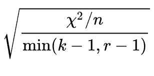
In this formula:
- x2 is the chi-square test statistic,
- n is the number of samples, and
- k is the number of columns, r is the number of rows
We can see that the result of Cramer’s V is dependent on the sample size and the dimensions of the crosstab. Let’s take a look at how we can calculate the test in Python!
How to Calculate Cramer’s V in Python
In this section, you’ll learn how to calculate Cramer’s V in Python using the SciPy library. To follow along, I have put together a sample dataset that measures job satisfaction alongside employee tenure.
| Job Satisfaction | Less Than 5 Years | More Than 5 Years |
|---|---|---|
| Satisfied | 45 | 50 |
| Neutral | 60 | 30 |
| Dissatisfied | 95 | 25 |
We can load this as a Pandas DataFrame as shown below:
import scipy.stats as stats
import pandas as pd

cross_tab = pd.DataFrame({
    'Less than 5 Years': [45, 60, 90],
    'More than 5 Years': [50, 30, 25]
}, index=['Satisfied', 'Neutral', 'Dissatisfied'])
We can first run a chi-square test of independence to see whether the two variables are independent of one another or not. This will let us know whether we should calculate Cramer’s V or not.
# Calculating the Chi-Square Test of Independence
x2, p, *_ = stats.chi2_contingency(cross_tab, correction=False)
print(p)

# Returns: 1.6865029961169425e-05
We can see that our p-value is less than 0.05, so we reject the null hypothesis that the two variables are independent. (Note, your threshold may be different in this case)
We can now calculate Cramer’s V. Let’s develop a custom function for this:
# Writing a Custom Function for Cramer's V
def cramers_v(cross_tab):
    X2 = stats.chi2_contingency(cross_tab, correction=False)[0]
    phi2 = X2 / cross_tab.sum().sum()
    n_rows, n_cols = cross_tab.shape
    return (phi2 / min(n_cols - 1, n_rows - 1)) ** 0.5
In the function above, we first calculate our chi-square test statistic. We then divide that by our number of samples (which is assumed to be a Pandas DataFrame or a NumPy array). We then unpack the shape of our data to get the number of rows and columns. Finally, we calculate Cramer’s V by dividing phi2 by the minimum of the smaller dimension minus 1. We return the square root value.
Let’s see what this returns for our sample dataset:
# Calculating Cramer's V
v = cramers_v(cross_tab)
print(v)

# Returns: 0.270681464861348
We can see that this returns 0.27.
Using SciPy to Calculate Cramer’s V
SciPy has a built-in function for calculating Cramer’s V, which simplifies the entire process. Let’s take a look at how we can use the association() function for this:
# Using SciPy to Calculate Cramer's V
v = stats.contingency.association(cross_tab)
print(v)

# Returns: 0.270681464861348
We can see that by passing our crosstab into the function, that we return the same value. This simplifies our implemetation quite a bit and allows us to ensure that we are using a well-tested function.
Now that you know how to calculate Cramer’s V, let’s take a look at how we can interpret the value.
How to Interpret Cramer’s V in Python
You may recall that the value for Cramer’s V ranges from 0 to 1, where
- 0 indicates that there is no association between the two variables, and
- 1 indicates that there is a strong association between the two variables.
However, the degrees of freedom of a dataset play a pivotal role in determing how associated two variables may be. For example, a larger crosstab will reduce the value of Cramer’s V – meaning that we can expect a smaller value, even for higher associations.
This academic paper provides a helpful illustration of how to interpret the association.
| Degrees of freedom | Small | Medium | Large |
|---|---|---|---|
| 1 | 0.10 | 0.30 | 0.50 |
| 2 | 0.07 | 0.21 | 0.35 |
| 3 | 0.06 | 0.17 | 0.29 |
| 4 | 0.05 | 0.15 | 0.25 |
| 5 | 0.04 | 0.13 | 0.22 |
In this case, the degrees of freedom as the minimum value of (# of rows – 1, # of columns -1). In our example, we would have min(2-1, 3-1), which would be a degree of freedom of 1. We can see that our Cramer’s V of 0.27 is on the higher end of small association, leading us to infer that there may be a decent amount of association between the two variables.
Conclusion
In conclusion, Cramer’s V serves as a valuable metric for assessing the strength of association between two nominal variables, providing insights into their relationship beyond mere independence. In this guide, you learned how the statistic is calculated, how you can use Python to calculate it, and how to interpret it. Cramer’s V serves as a great post-hoc test to the chi-square test of independence.
Additional Resources
To learn more about related topics, check out the tutorials below: