How to Remove Outliers in Python

When working in machine learning models, cleaning your data is a critical step that can make or break the success of your models. One of the most important data cleaning techniques you can develop as a data analyst or data scientist is identifying and removing extreme values. In this tutorial, you’ll learn how to remove outliers from your data in Python.

Extreme values are often called outliers. Outliers sit outside of the range of what is normally expend of your data and are generally unlike the rest of your data. Because of this, failing to remove outliers from your dataset can lead to poor performance of your model.

By the end of this tutorial, you’ll have learned how to do the following:

• Identify whether or not outliers exist in your dataset,
• Remove outliers using Python from your dataset,
• How to use different methods, including z-scores and interquartile ranges to identify and remove outliers, and
• How to automate the removal of outliers using Sci-kit Learn

What are outliers in data?

An outlier is a data record, or observation, that is different from other observations. To elaborate on this, an outlier is a rare occurrence which does not fit in the data.

Outliers can occur for many different reasons. For example, data may be entered in correctly (or be measured incorrectly from the get-go). Similarly, data may have been corrupted somewhere along the way. However, in some cases, outliers can be true data points. For example, Lionel Messi is an outlier in soccer.

While in this tutorial, we’ll explore how to identify and remove outliers, it’s often important to get a sense of whether a data point is a valid outlier or a product of entry errors.

Creating a Test Dataset

For the purposes of this tutorial, we’ll create a sample dataset. We’ll make a relatively normal distribution but also include a number of outliers to better understand what’s going on with our code. Let’s create our dataset and then visualize it:

# Creating a Normal Distribution With Some Outliers
import numpy as np
import seaborn as sns
import matplotlib.pyplot as plt
from scipy.stats import zscore

# Generating random normal data with outliers
np.random.seed(42)
mean = 5
std_dev = 2.5
num_samples = 1000

# Creating normal data
normal_data = np.random.normal(mean, std_dev, num_samples)

# Introducing outliers
num_outliers = 10
outlier_values = np.random.uniform(low=15, high=20, size=num_outliers)
data_with_outliers = np.concatenate((normal_data, outlier_values))

print(data_with_outliers[:5])

# Returns:
# array([6.24178538, 4.65433925, 6.61922135, 8.80757464, 4.41461656])

In the code block above, we used NumPy to create a normal distribution. We then added a number of outliers to the dataset so that we have some data points to work with.

Let’s now use a boxplot to visualize our data. Boxplots are helpful when we want to get a good sense of our distribution, by showing highlights of our descriptive statistics and values that extend past 1.5x the interquartile range values.

For this, we’ll use Seaborn, which allows us to easily visualize our data. We’ll use Matplotlib to add some customizations, such as titles:

# Visualize outliers in the 'sepal width (cm)' feature using a boxplot
plt.figure(figsize=(8, 6))
sns.boxplot(x=data_with_outliers)
plt.title('Sample Data in a Boxplot')
plt.show()

When we run the code above, we return the following visualization:

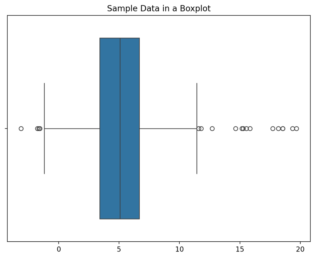
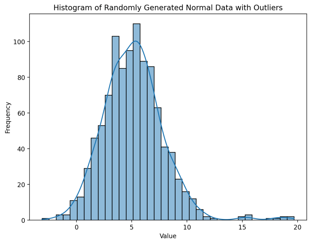
We can see that most of the data are centred around the mean but that there are some values that are beyond the extremes. Let’s take another look at how we can visualize the data using a histogram:

# Plotting histogram for the data with outliers
plt.figure(figsize=(8, 6))
sns.histplot(data_with_outliers, kde=True)
plt.title('Histogram of Randomly Generated Normal Data with Outliers')
plt.xlabel('Value')
plt.ylabel('Frequency')
plt.show()

This returns the visualization below:

I have shown two different visualizations here deliberately:

1. The boxplot shows us that we have extreme values (the dots on either end of the visualization), and
2. The histogram shows us that we have a relatively normal distribution, aside from the extreme values.

Many of the methods in this tutorial will assume that the data are normally distributed, so it’s a good thing to have in mind. Let’s now take a look at our first method, the standard deviation method, to identify and remove outliers from our data.

Using Z-Scores or Standard Deviations to Remove Outliers

One of the simplest ways of removing outliers from your data is to use z-scores or standard deviations. This assumes that your data are normally distributed (or Gaussian). This allows us to easily set thresholds for identifying outliers of where we expected rare values to sit.

What’s great about the normal distribution is that it allows us to easily identify where certain percentages of values will sit in a sample.

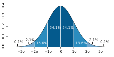
What we can see from the image above is that if our data is normally distributed, then we can easily measure percentage of data that will fall within a set number of standard deviations. More specifically:

• 68% of data will fall within 1 standard deviation from the mean,
• 95% of data will fall within 2 standard deviations from the mean, and
• 99.7% of data will fall within 3 standard deviations from the mean

This means that we can quantify how likely it is that a data point is expected to exist or not, based on the distribution. For example, if we know that a data point is more than 3 standard deviations away from the mean, there’s a less than 0.3% chance of it being in the sample.

Identifying Outliers with Z-scores in Python

The more standard deviations a data point is away from the mean, the less likely it is to occur. Because of this, we can set a threshold to identify our outliers in.

An easy way to do this is to use z-scores which quantify the number of standard deviations away from the mean a data point is. Because of this, we can say any data point with a value of greater than 3 z-scores is presumed to be an outlier and investigate it further. Let’s see what this looks like in Python:

# Getting z-scores from our data
from scipy.stats import zscore
zscores = zscore(data_with_outliers)

# Identifying Outliers with Z-scores
threshold = 3
outliers = data_with_outliers[np.abs(zscores) > threshold]

print("Detected outliers using Z-scores:")
print(outliers)

# Returns:
# Detected outliers using Z-scores:
# [14.63182873 -3.10316835 15.83741291 15.5228392  18.18215125 18.53237863
#  15.15793072 19.68106123 15.25985642 17.70648168 18.5453026  19.35484562]

In the code block above, we first imported the zscore() function from scipy. We then passed our array into the function which returned an array of z-scores. We then used boolean indexing to filter out our non-outlier data by selecting only records that are above the threshold.

We can see that this method identified 12 outliers in our data. At this point, you could take a closer look at the data to see what may be causing them to be outliers.

Let’s now take a look at removing outliers using z-scores.

Removing Outliers with Z-scores in Python

Now that we have identified the outliers in our dataset, we can simplify removing all of them. In order to do this, we can again use indexing on the dataset, but simply reverse the filtering.

# Removing Outliers with Z-scores
non_outliers = data_with_outliers[np.abs(zscores) <= threshold]

print(f'Data before removing outliers: {len(data_with_outliers)}')
print(f'Data after removing outliers: {len(non_outliers)}')

# Returns:
# Data before removing outliers: 1010
# Data after removing outliers: 998

In the code block above, we switched our indexing condition to include only values where the z-score is equal to or less than 3. We then checked the size of our dataset and were able to see that our 12 outlier data points were removed.

Using Interquartile Ranges to Remove Outliers

When working with non-normal data, using the interquartile range method can be a helpful approach to identifying outliers in our data.

But, what is the interquartile range? The interquartile range is the difference between the 75th and 25th percentile in the data. Recall our boxplot from earlier? This is the box in the boxplot.

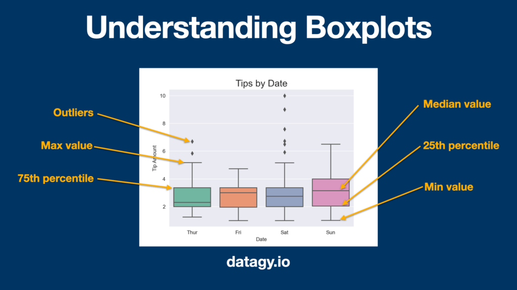
The image above shows how to interpret box plots. The box itself represents the data from the 25th to the 75th percentile (or the interquartile range). The line in the middle represents the 50th percentile, or the median. The whiskers of the plot in most cases represent the IQR value times 1.5 subtracted from the top and bottom of the box.

We can also see that the boxplot highlights some outliers in the data using markers. How are these outliers determined?

Outliers in boxplots or using the interquartile method are determined by values that sit outside of the following criteria:

• Greater than Q3 + 1.5 * IQR, or
• Less than Q1 - 1.5 * IQR

Identifying Outliers with Interquartile Ranges in Python

We can use what we learned above to create some code that allows us to find these values programatically. Let’s take a look at what this looks like:

# Calculate IQR
Q1 = np.percentile(data_with_outliers, 25)
Q3 = np.percentile(data_with_outliers, 75)
IQR = Q3 - Q1

# Define outlier boundaries using IQR method
lower_bound = Q1 - 1.5 * IQR
upper_bound = Q3 + 1.5 * IQR

# Detect outliers using IQR method
outliers_iqr = data_with_outliers[(data_with_outliers < lower_bound) | (data_with_outliers > upper_bound)]

print("Detected outliers using IQR:")
print(outliers_iqr)

# Returns:
# Detected outliers using IQR:
# [-1.54936276 11.80042292 14.63182873 -3.10316835 12.69720202 -1.74221661
#  -1.62742452 11.58095516 15.83741291 15.5228392  18.18215125 18.53237863
#  15.15793072 19.68106123 15.25985642 17.70648168 18.5453026  19.35484562]

Let’s break down what we did in the code block above:

1. We calculated the interquartile range by subtracting the first quartile from the third quartile
2. We then set lower and upper bounds by using the formulas we previously defined
3. We then created an or condition index by including only data that fall below our lower bound or above our upper bound

By printing out our values, we can see that we have 18 outliers using this method. Why is this number different our previous example? Put simply, because we’re using different criteria for identifying our outliers.

In the following section, we’ll explore how to remove outliers using the interquartile range method.

Removing Outliers with Interquartile Ranges in Python

Removing outliers using this method is very similar to our previous method. We can simply reverse the indexing that we used to identify our outliers. By doing this, we select only the data that hasn’t been identified as an outlier. Let’s take a look at what this looks like:

# Removing Outliers with IQR
non_outliers = data_with_outliers[(data_with_outliers >= lower_bound) & (data_with_outliers <= upper_bound)]

print(f'Data size before removal: {len(data_with_outliers)}')
print(f'Data size after removal: {len(non_outliers)}')

# Remove:
# Data size before removal: 1010
# Data size after removal: 992

By applying our indexing, we were able to remove the 18 outliers that we previously identified. Again, it’s not a good idea to blindly remove outliers but rather to investigate prior to removing them.

In the following section, you’ll learn how to use Sklearn to automatically identify and remove outliers.

Identify and Remove Outliers Automatically with Sklearn

In this section, we’ll explore how to identify and remove outliers automatically, using the popular Sci-kit Learn library. For this, we’ll make use of the LocalOutlierFactor class, which is used to find data points that are further away from others.

This works best for data that has fewer features. As the number of features increases, this can become less reliable.

The method works by assigning a score to each data point based on how isolated the data point is. When data have a higher score, they are identified to be outliers.

Let’s take a look at how this method works:

# Using Sklearn to Automatically Identify and Remove Outliers
from sklearn.neighbors import LocalOutlierFactor

outlier_factor = LocalOutlierFactor()
outliers = outlier_factor.fit_predict(data_with_outliers.reshape(-1, 1))

outliers_mask = data_with_outliers != outliers
outliers_removed = data_with_outliers[outliers_mask]
print(len(outliers_removed))

Let’s break down what we did in the code block above:

1. We imported the LocalOutlierFactor class and instantiated it
2. We then applied the .fit_predict() method, passing in our dataset
3. We then created a boolean mask to identify which records passed the threshold of not being outliers
4. Finally, we filtered these out by applying the mask as an index

While this approach is fast, it abstracts a lot of the process. This can be helpful if you’re just testing things out but can be tricky if you need to understand the ins and outs of your process. To learn more about the Local Outlier Factor class, check out the official documentation.

Conclusion

In the realm of machine learning models, data cleaning stands tall as a pivotal phase influencing the triumph or downfall of your models. Within this domain, the identification and eradication of extreme values emerge as an indispensable skill set for data analysts and scientists. This tutorial proficiently delves into the removal of outliers from datasets using Python. By traversing through methodologies like z-scores, interquartile ranges, and the automation prowess of Sci-kit Learn, it illuminates the path toward robust data preprocessing.

Outliers, often considered anomalies, linger outside the normal spectrum of dataset values, exerting potential harm on model performance if left unattended. The tutorial’s comprehensive breakdown vividly illustrates their impact, underlining the necessity of meticulous outlier identification and discernment. By crafting a sample dataset, visualizing it through boxplots and histograms, and meticulously employing z-scores and interquartile ranges, this tutorial not only imparts practical knowledge but also instills the importance of understanding data distributions before wielding outlier removal techniques. The emphasis on threshold customization and cautious outlier removal echoes the sentiment that their presence demands scrutiny—distinguishing between true data points and entry errors is paramount. Lastly, the introduction to Sklearn’s automated outlier detection offers a swift yet abstracted approach, ideal for quick assessments but with a caveat of potential oversights in intricate processes.