In this tutorial, you’ll learn how to calculate the Pearson Correlation Coefficient in Python. The tutorial will cover a brief recap of what the Pearson correlation coefficient is, how to calculate it with SciPy and how to calculate it for a Pandas Dataframe.
Being able to understand the correlation between different variables is a key step in understanding your data. It gives you substantial insight into how you may want to tune you machine learning models by understanding which variables have the highest and lowest degrees of correlation. This allows you to reduce dimensions found in a dataset, allowing your model to operate faster.
The Quick Answer: Use df.corr()
# Use Pandas .corr() to Calculate Pearson's r
df.corr()

# Returns:
#           English   History
# English  1.000000  0.930912
# History  0.930912  1.000000
Table of Contents
Pearson Correlation Coefficient Overview
The Pearson correlation coefficient, often referred to as Pearson’s r, is a measure of linear correlation between two variables. This means that the Pearson correlation coefficient measures a normalized measurement of covariance (i.e., a value between -1 and 1 that shows how much variables vary together).
The table below shows how the values of r can be interpreted:
Value of r | Linear Association Between Variables |
|---|---|
| +1 | Complete positive correlation |
| +0.8 | Strong positive correlation |
| +0.6 | Moderate positive correlation |
| 0 | No correlation |
| -0.6 | Moderate negative correlation |
| -0.8 | Strong negative correlation |
| -1 | Complete negative correlation |
rWhat do the terms positive and negative mean? Positive correlation implies that as one variable increases as the other increases as well. Inversely, a negative correlation implies that as one variable increases, the other decreases.
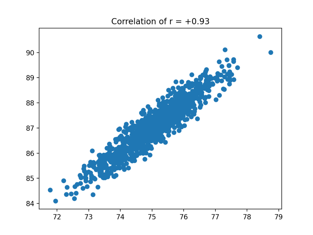
The visualization below shows a value of r = +0.93, implying a strong positive correlation:

In the next section, we’ll start diving into Python and Pandas code to calculate the Pearson coefficient of correlation.
Loading a Sample Pandas Dataframe
Let’s take a look at how we can calculate the correlation coefficient. To do this, we’ll load a sample Pandas Dataframe. If you have your own dataset, feel free to follow along with that. If you want to follow along line by line, copy the code below to get started:
# Loading a Sample Pandas Dataframe
import pandas as pd
df = pd.read_excel('https://github.com/datagy/mediumdata/raw/master/Scores.xlsx')

print(df.head())

# Returns:
#      English    History
# 0  74.573424  86.496775
# 1  75.115299  86.801171
# 2  75.691345  87.981466
# 3  73.888714  85.411392
# 4  75.015225  86.812830
We can see that we have two columns: one with grades for English and another with grades for History. Imagine that these represent grades from different students and we want to explore any type of correlation between the two.
How to Calculate Pearson Correlation Coefficient in Pandas
Pandas makes it very easy to find the correlation coefficient! We can simply call the .corr() method on the dataframe of interest. The method returns a correlation matrix that shows the coefficient of correlation between different variables.
Let’s take a look at what this looks like:
# Calculating a correlation matrix
print(df.corr())

# Returns:
#           English   History
# English  1.000000  0.930912
# History  0.930912  1.000000
What does this matrix tell us? You’ll notice that the columns of our dataframe are represented using both rows and columns. The row-column intersection represents the coefficient of correlation between two variables. Because of this, the diagonal line will always be 1 (since it compares a variable to itself). Similarly, the matrix will be a mirror along the diagonal line.
Many people take these matrices and visualize them using heat maps. You can learn about this process in this in-depth tutorial, which will show you different formatting options.
In order to access just the coefficient of correlation using Pandas we can now slice the returned matrix. The matrix is of a type dataframe, which can confirm by writing the code below:
# Getting the type of a correlation matrix
correlation = df.corr()
print(type(correlation))

# Returns: <class 'pandas.core.frame.DataFrame'>
Because our correlation matrix is a dataframe, we can use the .loc accessor to access data within it.
Say we wanted to find the correlation coefficient between our two variables, History and English, we can slice the dataframe:
# Getting the Pearson Correlation Coefficient
correlation = df.corr()
print(correlation.loc['History', 'English'])

# Returns: 0.9309116476981859
In the next section, you’ll learn how to use numpy to calculate Pearson’s r.
How to Calculate Pearson’s r with Numpy
Similarly, Numpy makes it easy to calculate the correlation matrix between different variables. The library has a function named .corrcoef(). We can pass in two columns from a Pandas Dataframe to calculate the correlation matrix between them.
Let’s see how we can use the function to calculate Pearson’s r:
# Calculate
import pandas as pd
import numpy as np

df = pd.read_excel('https://github.com/datagy/mediumdata/raw/master/Scores.xlsx')

corr = np.corrcoef(df['History'], df['English'])
print(corr)

# Returns:
# [[1.         0.93091165]
#  [0.93091165 1.        ]]
We can see that a correlation matrix between the two variables is returned.
To learn more about the NumPy .corrcoef() function, check out the official documentation here. In the next section, you’ll learn how to use SciPy to calculate the Pearson Correlation Coefficient.
How to Calculate Pearson Correlation Coefficient in SciPy
While Pandas makes it easy to calculate the correlation coefficient, we can also make use of the popular SciPy library. We can use the scipy.stats.pearsonr() function to calculate Pearson’s r. The function takes two parameters, an x and a y value.
Let’s take a look at how we can pass in our dataframe columns by selecting them.
# Calculate Pearson's r with scipy
import pandas as pd
import scipy.stats as stats

df = pd.read_excel('https://github.com/datagy/mediumdata/raw/master/Scores.xlsx')

r = stats.pearsonr(df['History'], df['English'])
print(r)

# Returns: (0.9309116476981856, 0.0)
We can see that this returns a tuple of values:
- r: Pearson’s correlation coefficient
- p-value: long-tailed p-value
In order to access the coefficient, we can simply index the tuple:
df = pd.read_excel('https://github.com/datagy/mediumdata/raw/master/Scores.xlsx')

r = stats.pearsonr(df['History'], df['English'])
print(r[0])

# Returns: 0.9309116476981856
Conclusion
In this tutorial, you learned how to calculate the Pearson correlation of coefficient using Pandas and SciPy. Being able to calculate Pearson’s r is an important step in better understanding your data. As the scope of your dataset grows in machine learning, being able to find strongly correlated variables allows you to remove those that aren’t correlated.
Being able to remove features that don’t add value to your machine learning models is known as a parameter reduction. This is just a small part of the puzzle and does require more insight before overly relying on this method.
To learn more about the SciPy .pearsonr() function, check out the official documentation here.
Additional Resources
To learn more about related topics, check out the resources below:


Pingback: How to Calculate Mean Squared Error in Python • datagy