Linear Regression in PyTorch

In this tutorial, you’ll learn how to create linear regression models in PyTorch. Linear models are one of the foundational building blocks of deep learning models. Understanding how to build linear models in PyTorch can allow you to solve many different types of problems.

By the end of this tutorial, you’ll have learned the following:

• How to load regression data using Scikit-Learn
• How to prepare your data to build linear models in PyTorch using Datasets and DataLoaders
• How to build a linear regression model class
• How to train and evaluate your linear regression model in PyTorch

Loading a Regression Dataset

Let’s start by loading a sample dataset we’ll use for this tutorial. To build linear regression datasets in Python, we can use the Scikit-Learn library. Let’s see we can build a simple linear model using the make_regression() function:

# Loading a Sample Dataset
from sklearn.datasets import make_regression
import matplotlib.pyplot as plt

bias = 10
X_numpy, y_numpy, coef = make_regression(
    n_samples=5000,
    n_features=1,
    n_targets=1,
    noise=5,
    bias=bias,
    coef=True,
    random_state=42
)

In the code block above, we defined a linear regression dataset using the make_regression() function. In it, we passed in the number of samples, features, and targets. To keep things simple, we created a dataset that only had one feature and one target. This means that the dataset has only one x variable and only one corresponding y variable.

We added in a few more parameters:

• noise= defines the standard deviation of the gaussian noise applied to the output
• coef= indicates that we want to return the coefficients of the underlying linear model
• random_state= allows us to reproduce our results

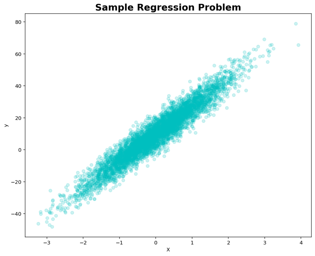
Let’s now use Matplotlib to visualize our data. Matplotlib is the defacto data visualization library available in Python, allowing us to customize visualizations to a great degree.

# Create a Scatter Plot
fig, ax = plt.subplots(figsize=(10, 8))
ax.scatter(X_numpy, y_numpy, c='c', marker='o', alpha=0.2)

# Set labels and title
ax.set_xlabel('X')
ax.set_ylabel('y')
ax.set_title('Sample Regression Problem', size=18, weight='bold')

# Show the plot
plt.show()

In the code block above, we used Matplotlib to create a scatter plot. We plotted our x and y variables and gave the plot a title. This returned the following image:

We can see that the data follows a linear trend. Let’s now see how we can prepare our data for creating a linear model in PyTorch.

Preparing Data for Linear Regression in PyTorch

PyTorch allows you to add structure to your deep learning problems by using Datasets and DataLoaders:

• PyTorch Datasets allow you to structure your datasets in a way that provides access to individual items, facilitate transformations and integrate with other PyTorch workflows
• PyTorch DataLoaders allow you to batch your data for training and evaluating in memory-efficient ways

Creating a PyTorch Dataset

Let’s take a look at how we can create a PyTorch Dataset based on our data:

# Creating a PyTorch Dataset
import torch
import torch.nn as nn
import torch.optim as optim
from torch.utils.data import DataLoader, Dataset, random_split

# Define a Dataset
class RegressionDataset(Dataset):
    def __init__(self, X, y):
        super().__init__()
        self.X = torch.from_numpy(X_numpy.astype('float32'))
        self.y = torch.from_numpy(y_numpy.astype('float32'))

    def __len__(self):
        return len(self.X)
    
    def __getitem__(self, index):
        return self.X[index], self.y[index].unsqueeze(0)
    
dataset = RegressionDataset(X_numpy, y_numpy)

In the code block above, we defined our RegressionDataset class, inheriting from the Dataset class. This means that we need to define a __len__ and a __getitem__ method. In our __init__ method, we first convert our data to Tensors, allowing PyTorch to better work with our data. We then implement simple methods to return the length of our data and ways in which we can index our dataset.

Let’s now take a look at how we can split our data into training and testing data.

# Splitting Our Dataset into Training and Testing
train_dataset, test_dataset = random_split(dataset, lengths=[0.8, 0.2])

In the code block above, we used the PyTorch random_split function to create training and testing datasets. We passed in our dataset and the proportions of the split that we want to use.

Creating a PyTorch DataLoader

The PyTorch DataLoader class is an important tool to help you prepare, manage, and serve your data to your deep learning networks. Most importantly, it’s used to batch your data.

We can define both a testing data loader and a training loader, allowing to easily pass our data in our model. Let’s see how we can do this in Python:

# Create DataLoaders
train_loader = DataLoader(
    dataset=train_dataset,
    batch_size=64,
    shuffle=True
)

test_loader = DataLoader(
    dataset=test_dataset,
    batch_size=64,
    shuffle=True
)

Both of the DataLoaders are defined similarly: we set the batch size to 64 and ask PyTorch to shuffle our data. Now that our data is prepared, we can move into building our linear regression model.

Defining a Simple Linear Regression Model in PyTorch

PyTorch uses classes to define the structure of deep learning models, inheriting from the nn.Module module. These classes help capture the complexity of our datasets and make using our models quite simple. The main requirement of developing our classes is that they implement a forward() method.

Let’s take a look at how we can define a linear regression deep learning model in PyTorch:

# Define Linear Regression Class
class LinearRegressionSimple(nn.Module):
    def __init__(self, in_features=1, out_features=1):
        super().__init__()
        self.linear = nn.Linear(
            in_features=in_features, 
            out_features=out_features
            )

    def forward(self, x):
        return self.linear(x)

In the code block above, we implemented our linear regression model class. There’s quite a bit going on, so let’s break this down, step by step:

1. We defined our class and inherited from nn.Module. This allows our class to easily interact with many of the different elements in PyTorch, such as our training loop.
2. We implement the __init__ method. The first thing we do is run the super() function, which provides access to the methods and attributes that we just inherited. We also allow passing in our i-in_features and out_features, which are set to 1 by default.
3. We then define our self.linear callable, which implements the nn.Linear() function.

Because our dataset has only a single feature and a single target, both our in_features and out_features are equal to 1. As the complexity of your data changes, be mindful of how you need to adapt your model class.

We can now instantiate linear regression model by instantiating the class:

# Instantiating our Model
model = LinearRegressionSimple()

Let’s now move on to defining our loss function and optimizers.

Creating Loss Functions and Optimizers in PyTorch

PyTorch optimizers are essential as they provide a range of algorithms that enable efficient parameter updates during the training process, allowing deep learning models to converge towards optimal solutions. Similarly, PyTorch criterion functions play a crucial role by defining the objective or loss function, enabling the quantification of model performance and guiding the optimization process towards the desired outcome.

Let’s see how we can add both a loss function (criterion) and an optimizer:

# Adding Loss Function and Optimizer
criterion = nn.MSELoss()
optimizer = optim.SGD(params=model.parameters(), lr=0.001)

In the code block above, we first defined our loss function by instantiating the MSELoss class. This allows us to use the mean squared error when calculating our model’s performance. The R-squared value is a normalized version of the mean squared error.

Similarly, we defined our optimizer. We used stochastic gradient descent in this case, but you can experiment with others. We passed in our model’s parameters by using the .parameters() method and also passed in a learning rate of 0.001. This learning rate is a hyperparameter, meaning you can play around with it, but 0.001 is a good starting point.

We’re finally ready to build our training and validation loop! Let’s dive into this in the following section.

Training a Linear Regression Model in PyTorch

It’s common in PyTorch to define training and validation functions for your deep learning models, which you can then loop over as you train your model. Before we define our loops, let’s set up a few pieces.

The first thing we’ll want to do is define a device that we have access to. To make our code more agnostic, we can define a variable that checks whether a GPU is available. If it is, then we use it – otherwise, we’ll use our CPU:

# Defining our device
device = 'cuda' if torch.cuda.is_available() else 'cpu'

In the code block above, we use the ternary operator to define what type of device we want to use for our deep-learning model.

Let’s now define two empty lists that we can use to track our losses. This will allow us to later visualize the losses of our model as it trains.

# Setting up lists to track losses
train_losses = []
val_losses = []

Now, let’s dive into developing some functions to train and test our model. First, we’ll develop our train() function, which will help encapsulate our training complexity. While you may see this done in practice without a dedicated function, I find this process much cleaner.

# Defining a Training Function
def train(model, train_loader, criterion, optimizer, epoch, num_epochs):
    model.train()
    train_loss = 0.0

    for inputs, targets in train_loader:
        inputs = inputs.to(device)
        targets = targets.to(device)

        # Forward pass
        outputs = model(inputs)
        loss = criterion(outputs, targets)
        optimizer.zero_grad()
        train_loss += loss.item()

        # Backward pass and optimization
        loss.backward()
        optimizer.step()

    avg_loss = train_loss/len(train_loader)
    print(f'Epoch [{epoch + 1:03}/{num_epochs:03}] | Train Loss: {avg_loss:.4f}')
    train_losses.append(train_loss/len(train_loader))

At the beginning of the function, the model is set to training mode using model.train(). This ensures that certain layers within the model, such as dropout or batch normalization, behave correctly during the training process.

The function then enters a loop that iterates over the mini-batches of the training data. Each mini-batch consists of a batch of input data and their corresponding target labels. The inputs and targets are moved to the appropriate device, such as a GPU, using inputs = inputs.to(device) and targets = targets.to(device) for faster computation if available.

Before computing the gradients in the backward pass, optimizer.zero_grad() is called to clear the gradients of the model’s parameters. This step ensures that the gradients are not accumulated from previous iterations. The model performs a forward pass by passing the input data through it to generate predictions. The loss between the predicted outputs and the target labels is computed using the specified loss function (criterion).

The current batch’s loss value is then added to the running total of the training loss for the current epoch using train_loss += loss.item(). This accumulation allows the function to keep track of the overall training loss for the epoch.

Backpropagation is performed next by calling loss.backward(), which computes the gradients of the loss with respect to the model’s parameters. Finally, the optimizer’s step() method is called to update the model’s parameters using the computed gradients. This step is crucial for optimizing the model and improving its performance.

Finally, the train_loss variable is reset to zero in preparation for the next set of mini-batches in the next iteration.

Now, let’s take a look at our validation function:

# Defining a Validation Function
def validate(model, val_loader, criterion, device):
    model.eval()
    val_loss = 0.0

    with torch.no_grad():
        for inputs, targets in val_loader:
            inputs = inputs.to(device)
            targets = targets.to(device)

            # Forward pass
            outputs = model(inputs)
            loss = criterion(outputs, targets)
            val_loss += loss.item()

    avg_loss = val_loss / len(val_loader)
    print(f'Validation Loss: {avg_loss:.4f}')
    val_losses.append(avg_loss)

Let’s break down what the function does step by step. At the beginning of the function, the model is set to evaluation mode using model.eval(). This ensures that certain layers within the model, such as dropout or batch normalization, behave differently than during training.

The function then enters a loop that iterates over the mini-batches of the validation data. Each mini-batch consists of a batch of input data and their corresponding target labels. The inputs and targets are moved to the appropriate device, such as a GPU, using inputs = inputs.to(device) and targets = targets.to(device) for faster computation if available.

During each iteration of the loop, a forward pass is performed by passing the input data through the model to generate predictions. The loss between the predicted outputs and the target labels is computed using the specified loss function (criterion) with loss = criterion(outputs, targets). The current batch’s loss value is added to the running total of the validation loss using val_loss += loss.item().

After the loop, the average validation loss is computed by dividing the accumulated loss by the number of mini-batches (len(val_loader)). The accuracy is calculated by dividing the number of correctly predicted samples by the total number of samples. The validation loss and accuracy are then printed to provide an overview of the model’s performance on the validation dataset.

Let’s now take a look at how we can use these functions to train and validate our model:

# Running our training loop
num_epochs = 30
model.to(device)
for epoch in range(num_epochs):
    train(model, train_loader, criterion, optimizer, epoch, num_epochs)
    validate(model, test_loader, criterion, device)

In the code block above, we define a new variable to define how many epochs we want to run through our code. An epoch is the number of times every element of data should be seen during training.

We then move our model to our device. Finally, we loop over our training and validation functions 30 times. Because we’re printing our results as we go, we can see the results reflected.

Epoch [001/030] | Train Loss: 362.3502
Validation Loss: 337.1006
Epoch [002/030] | Train Loss: 289.3616
Validation Loss: 266.5897
...
Epoch [029/030] | Train Loss: 25.9918
Validation Loss: 27.0739
Epoch [030/030] | Train Loss: 25.9491
Validation Loss: 26.8830

We can see that the loss starts quite high and then decreases.

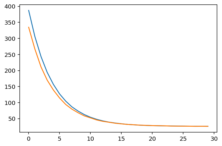
Since we’ve been keeping track of our model’s performance, we can now use Matplotlib to plot our data. We’ll use the plot() function to create a line plot.

# Creating a Line Chart of Our Data
plt.plot(range(len(train_losses)), train_losses, val_losses)

Plotting our losses returns the visualization below:

We can see that the model’s performance improves rapidly and then slows down. This is expected, but it’s reassuring to see our validation loss continuing to decrease as well. This indicates that our model isn’t overfitting.

We can also now access both the weight and bias of our dataset. Earlier, when we defined our dataset, we created them with a bias of 10. We also defined a coef variable, which contains our model’s weight (which is equal to 16.82365791).

We can access the model’s weight and bias to see how accurate it is:

# Printing the Model's Weight and Bias
print(f'{model1.linear.bias=}')
print(f'{model1.linear.weight=}')

# Returns:
# model1.linear.bias=Parameter containing:
# tensor([9.6979], requires_grad=True)
# model1.linear.weight=Parameter containing:
# tensor([[16.4274]], requires_grad=True)

We can see that while close, they’re not identical. This is because we’ve defined a very simple architecture and also added noise to our dataset.

Next Steps

So, we’ve trained a model and it performs well. But what can we do next to improve its performance? We can add more layers (especially more hidden layers), for example. Similarly, we can add activation functions that allow us to capture more complexity in your data. While our current dataset is quite simple, if we’re working with non-linear or more complex data, this can be an important next step.

Conclusion

This tutorial provided a comprehensive guide on how to create linear regression models in PyTorch. Linear models serve as fundamental building blocks in deep learning and understanding their implementation in PyTorch enables solving various problem types.

Throughout the tutorial, we covered the following key topics:

1. Loading a regression dataset using Scikit-Learn and visualizing the data using Matplotlib.
2. Preparing data for linear regression in PyTorch by creating a PyTorch Dataset class and splitting the dataset into training and testing sets.
3. Utilizing PyTorch DataLoaders to batch and shuffle the data efficiently.
4. Defining a simple linear regression model in PyTorch by creating a class that inherits from nn.Module and implements the forward() method.
5. Setting up the loss function (criterion) and optimizer using PyTorch’s MSELoss and SGD classes, respectively.
6. Training the linear regression model by iterating over training and validation loops, tracking the losses for evaluation.

By following this tutorial, you have gained the knowledge and practical skills necessary to create and train linear regression models in PyTorch. Linear regression serves as a fundamental technique in machine learning, and PyTorch’s flexibility and functionality make it a powerful framework for implementing such models.