PyTorch Convolutional Neural Networks (CNN)

In this guide, you’ll learn how to develop convolution neural networks (or CNN, for short) using the PyTorch deep learning framework in Python. Convolution neural networks are a cornerstone of deep learning for image classification tasks. Understanding how to develop a CNN in PyTorch is an essential skill for any budding deep-learning practitioner.

By the end of this guide, you’ll have learned the following:

• How to structure data for convolutional neural networks in PyTorch
• How to develop convolutional neural networks (CNN) in PyTorch
• How to understand the inner workings of convolutions and max pooling layers
• How to develop training and validation loops

This guide will work with you, step-by-step, through loading data, developing a model, training and evaluating a model, to using it for live inference:

Getting Started with CNNs in PyTorch

To start things off, let’s import our libraries and download the data that we’ll use. There are quite a few but don’t worry, they all serve a purpose. You’ll notice that we import some modules from PyTorch directly. This is done conventionally and will allow others to read your code more efficiently.

# Importing Libraries
import torch
import torch.nn as nn
import torch.optim as optim
from torch.utils.data import DataLoader, Dataset, random_split
import torchvision
from torchvision import transforms, datasets
import torch.nn.functional as F
torch.manual_seed(42)

from PIL import Image
from dataclasses import dataclass
import matplotlib.pyplot as plt
import random
import numpy as np

Now that we have our libraries imported, let’s work on downloading our data. I wanted to make this tutorial a bit different by using a custom dataset.

We’ll use a dataset to predict the hand shape of rock, paper, and scissors. All of the images are of my hands, which of course leads to a flawed dataset. For example, there’s little variation in lighting, background, and skin tone. The purpose here is not to develop a completely robust CNN, but show you how the underlying mechanics of building them in PyTorch.

You can download the files here as a zip file (which, if you want to use Python to unzip, you can!). The file contains a number of directories for each of our classes (or hand signals).

Preparing Data in PyTorch for CNNs

PyTorch uses classes to structure your deep-learning projects. Organizing your data into PyTorch Datasets and DataLoaders allows you to easily structure, access, and manipulate your datasets. In this section, we’ll use the dataset that you previously downloaded and organize them into abstracted datasets.

• PyTorch Datasets allow you to structure your datasets in a way that provides access to individual items, facilitate transformations and integrate with other PyTorch workflows
• PyTorch DataLoaders allow you to batch your data for training and evaluating in memory-efficient ways

Creating a PyTorch Dataset

Let’s now create a PyTorch Dataset class, which will allow us to access our data and iterate over it. The Dataset class is an abstract base class, requiring us to implement two methods:

1. __len__, which returns the length of our dataset, and
2. __getitem__, which allows us to index an item

Let’s take a look at how we can create a Dataset class with PyTorch:

# Define overall dataset class
class RPSDataset(Dataset):
    def __init__(self, data_dir, transform=None):
        self.data_dir = data_dir
        self.transform = transform
        self.dataset = datasets.ImageFolder(self.data_dir, transform=self.transform)

    def __len__(self):
        return len(self.dataset)

    def __getitem__(self, index):
        return self.dataset[index]

In the code block above, we first declare our class RPSDataset, which inherits from the Dataset class. We allow the class to take two parameters:

1. Our data directory, and
2. A transforms composition object, which defaults to None. This will allow us to preprocess our visualizations as the data are loaded.

In the __init__ method, we also create a self.dataset attribute, which uses the ImageFolder class to easily load our data directory. This assumes that the data directory is structured as below:

root/class1/aaa.png
root/class1/aab.png
...
root/class2/aaa.png
root/class2/aab.png
...

You’ll notice that the directory you previously downloaded already has the data structured in this way. Now, I had mentioned earlier that the dataset is not perfect. By transforming our data, we can add some variety to the pictures, allowing it to be a bit more robust.

Let’s take a look at how we can use PyTorch to define image transformations using the Compose class.

# Define the transforms to use
data_transforms = transforms.Compose([
    transforms.Resize((90, 90)),
    transforms.RandomHorizontalFlip(),
    transforms.RandomRotation(10),
    transforms.ColorJitter(brightness=0.1, contrast=0.1, saturation=0.1, hue=0.1),
    transforms.ToTensor(),
    transforms.Normalize((0.5, 0.5, 0.5), (0.5, 0.5, 0.5))
])

In the code block above, we define our transformations object by passing in a list of transforms. torchvision comes with a number of different transformations built in, allowing us to easily define transformations using a familiar API.

Now that we have a list of transformations defined, we can instantiate our dataset by passing both the directory and the transforms into the class:

# Instantiate a Dataset
dataset = RPSDataset('data/cnn/image_data/', transform=data_transforms)

Now that we have our dataset created, we can start working with it.

Exploring Our PyTorch Dataset

Once we have our dataset defined, we can actually dive into it and explore it. Because we defined a method that allows us to index the dataset, we can index the images directly:

# Exploring the Dataset
print(dataset[0])

# Returns:
# (tensor([[[-0.9529, -0.9529, -0.9529,  ..., -0.9529, -0.9529, -0.9529],
#           [-0.9529, -0.9529, -0.9529,  ..., -0.9529, -0.9529, -0.9529],
#           [-0.9529, -0.9529, -0.9529,  ..., -0.9529, -0.9529, -0.9529],
#           ...,
#           [-0.9529, -0.9529, -0.9529,  ..., -0.9529, -0.9529, -0.9529],
#           [-0.9529, -0.9529, -0.9529,  ..., -0.9529, -0.9529, -0.9529],
#           [-0.9529, -0.9529, -0.9529,  ..., -0.9529, -0.9529, -0.9529]]]),
#  0)

In the code block above, we accessed the first item in our dataset. Recall from defining our __getitem__ method that the method actually returns a tuple. You’ll notice in the code block above that we actually return a tuple containing the tensor information of our image and the class that is associated with it.

We can visualize the image using the code block below, by accessing the first item of that item:

# Visualizing a Sample Image
plt.imshow(dataset[0][0].numpy().transpose(1, 2, 0))

This returns the following image:

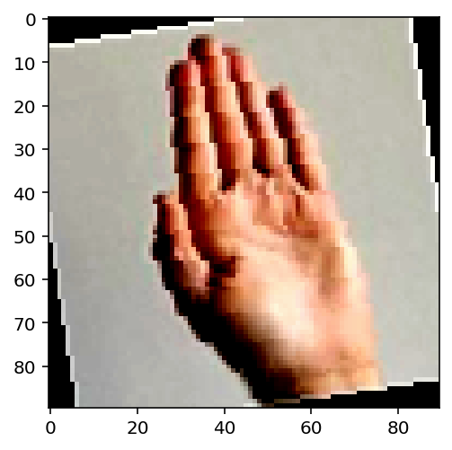
We can see that the image looks quite different than what we originally started working with. By including some randomness in how our dataset is transformed, we can make our dataset more robust.

Visually, we can see that class 0 refers to “paper”. But, how do we get access to this programmatically?

Because we inherit from the Dataset class, we get access to a ton of useful methods and attributes under the hood. For example, we can access the class to index mapping by using the .class_to_idx attribute.

# Get variables for Classes and Indices
classes_to_idx = dataset.dataset.class_to_idx
idx_to_classes = {v: k for k, v in classes_to_idx.items()}

In the code block above, we create a dictionary mapping our classes to our indices. We then used a dictionary comprehension to create a mapping of index to classes.

Splitting Our Dataset into Training and Testing

Before we dive into creating our deep learning model, let’s finish preparing our data. We can split our data into training and testing data, which allows us to test the model on data that the model hasn’t yet seen.

In order to do this, we can use the random_split() function, which accepts a dataset and a list of lengths. The list can either represent the number of records as integers or the proportion of the data as floats.

# Split into Train/Test Datasets
train_data, test_data = random_split(dataset, lengths=[0.8, 0.2])

In the code block above, we instantiated two variables, train_data and test_data. These variables are returned from the random_split() function, which creates an 80/20 split.

Now that we have our two datasets, we can create some DataLoaders that facilitate iterating over our data.

Creating a PyTorch DataLoader

The PyTorch DataLoader class is an important tool to help you prepare, manage, and serve your data to your deep learning networks. Because many of the pre-processing steps you will need to do before beginning training a model, finding ways to standardize these processes is critical for the readability and maintainability of your code.

Let’s create both a training data loader and a testing data loader:

# Defining Training and Testing DataLoaders
train_loader = DataLoader(train_data, batch_size=64, shuffle=True)
test_loader = DataLoader(test_data, batch_size=64, shuffle=True)

In the code block above, we created both of our DataLoaders. We asked PyTorch to create a batch size of 64 (meaning 64 images will be loaded at once) and that we want to shuffle our dataset.

Let’s now explore one of the data loaders, to get a sense of the dimensions that we’re working with:

# Exploring a DataLoader Batch
iterator = iter(train_loader)
imgs, labels = next(iterator)

print(f'Number of images: {len(imgs)}')
print(f'Number of labels: {len(labels)}')
print(f'Shape of images batch: {np.array(imgs).shape}')

# Returns:
# Number of images: 64
# Number of labels: 64
# Shape of images batch: (64, 3, 90, 90)

In the code block above, we first turned our training DataLoader into an iterable. We then created variables for our images and labels using the next() function, which accessed the first batch. From there, we printed out the following:

1. The number of images,
2. The number of labels, and
3. The shape of images in a batch.

Notice here, that the shape of our batch is represented by 64 images (our batch size), 3 dimensions (because our images are RGB), and a height and width of 90.

Now that our data and loaders are defined and loaded, let’s work on defining our actual convolution neural network!

Defining a Convolutional Neural Network in PyTorch

PyTorch allows you to define convolution neural networks using classes that inherit from the nn.Module class, which defines many helpful methods and attributes for neural networks.

Within our classes, we need to define a forward() method, which allows for data to propagate through the model. Let’s take a look at our model class:

class RPSClassifier(nn.Module):
    def __init__(self):
        super(RPSClassifier, self).__init__()
        self.conv1 = nn.Conv2d(in_channels=3, out_channels=6, kernel_size=3)
        self.pool = nn.MaxPool2d(kernel_size=2, stride=2)
        self.conv2 = nn.Conv2d(in_channels=6, out_channels=16, kernel_size=5)
        self.fc1 = nn.Linear(16 * 20 * 20, 120)
        self.fc2 = nn.Linear(120, 84)
        self.fc3 = nn.Linear(84, 3)

    def forward(self, x):
        x = self.pool(F.relu(self.conv1(x)))
        x = self.pool(F.relu(self.conv2(x)))
        x = x.view(-1, 16 * 20 * 20)
        x = F.relu(self.fc1(x))
        x = F.relu(self.fc2(x))
        x = self.fc3(x)
        return x

There’s a lot going in the code block above. While on the surface this model looks complex, it’s actually quite small compared to other convolutional natural networks. Let’s break down what’s going in our model.

First, we use the super() function to instantiate any parent methods and attributes. Then, we define our model’s layers. The layers are broken down as below:

1. self.conv1 is a 2D convolutional layer, which takes 3 channels as input, returns 6 channels, and uses a kernel size of 3
2. Then, we define a self.pool layer which uses a max pooling layer to reduce the layer size using a kernel of 2.
3. self.conv2 is another 2D convolutional layer, which uses 6 channels as input (the output from our previous convolutional layer) and returns 16 channels. Similarly, the layer uses a kernel of 5 to find larger features.
4. Then, we define three linear layers. The input of our first linear layer is 16 (the number of channels) by 20 (the current width) by 20 (the current height). This reduces the deep convolutional layer into a linear model. The output is 120 nodes.
5. From there, we pass through two more linear layers. The first reduces the 120 nodes to 84. From there, we reduce it further to 3, which represents the number of classes that our model has.

In our forward() method, we allow our data to pass through the model. An important thing to note here is that we pass through each convolutional layer, passing the result through the max pooling layer. We then change the dimensions of our data using the view() method. Finally, we pass through our linear layers, applying the ReLU activation function to the first two layers’ outputs.

Let’s now instantiate our model, calling it model.

model = RPSClassifier()

One of the big things that stumps many newcomers to convolutional neural networks (and stumped me for a long time) is how the sizes change as the image traverses through the model. Let’s take a look at this in the following section.

Understanding Layer Sizes in PyTorch CNNs

In this section, we’ll explore how the layer sizes change in a convolutional neural network. Because these layer sizes determine the inputs and outputs of different layers, it’s a good idea to have a handle on them.

One way to do this is to recreate the layers one by one and print out the shapes. This is a great heuristic approach that allows you to understand the sizes as you go. Let’s take a look at what this looks like:

# Checking Sizes of Layers
conv1 = nn.Conv2d(3,6,3)
pool = nn.MaxPool2d(2,2)
conv2 = nn.Conv2d(6,16,5)
img_conv1 = conv1(dataset[0][0])
img_pool1 = pool(img_conv1)
img_conv2 = conv2(img_pool1)
img_pool2 = pool(img_conv2)

print(f'{img_conv1.shape=}')
print(f'{img_pool1.shape=}')
print(f'{img_conv2.shape=}')
print(f'{img_pool2.shape=}')

# Returns:
# img_conv1.shape=torch.Size([6, 88, 88])
# img_pool1.shape=torch.Size([6, 44, 44])
# img_conv2.shape=torch.Size([16, 40, 40])
# img_pool2.shape=torch.Size([16, 20, 20])

In the code block above, we defined our layers in the same way that we had before. We then passed a single image through these layers and then printed the sizes of the image at each layer.

Being able to see that last layer allows us to see the input size into the first linear layer. Here, we can see that we have (16, 20, 20), which then also gets multiplied by the number of channels (3).

Developing Custom Functions for Layer Sizes in Convolutional Neural Networks in PyTorch

A more structured approach for this is to develop custom functions that allow you to calculate the layer sizes. This is what we do in the code block below.

# Creating Functions to Calculate the Sizes
def conv2d_size(input_size, kernel_size, padding=0, stride=1, dilation=1):
    output_width = (input_size[0] + 2 * padding - dilation * (kernel_size - 1) - 1) // stride + 1
    output_height = (input_size[1] + 2 * padding - dilation * (kernel_size - 1) - 1) // stride + 1
    return output_width, output_height

def maxpool2d_size(input_size, kernel_size, stride=None, padding=0, dilation=1):
    if stride is None:
        stride = kernel_size  # Default stride is equal to kernel size
    
    output_width = (input_size[0] + 2 * padding - dilation * (kernel_size - 1) - 1) // stride + 1
    output_height = (input_size[1] + 2 * padding - dilation * (kernel_size - 1) - 1) // stride + 1
    
    return output_width, output_height

While this approach works well, it can be intimidating for folks just getting started. Because of this, I tend to recommend using the first approach and seeing the sizes one layer at a time. From there, you can move on to using the functions that give you a much deeper understanding.

Visualizing Convolutional Layers in PyTorch

PyTorch abstracts the complexities and intricacies of neural networks. Because of this, it can be easy to forget what makes convolutional neural networks so beautiful.

The key idea behind a convolutional layer is to use small filters (also known as kernels) to scan over the input data and perform element-wise multiplication and summation operations. These filters act as feature detectors, helping the model learn relevant patterns, edges, textures, and other visual characteristics from the input.

Here’s how a convolutional layer works:

1. Input: The input to a convolutional layer is a multi-dimensional array, typically representing an image or a feature map from the previous layer. For colored images, the input usually consists of three channels (red, green, and blue), while for grayscale images, there’s only one channel.
2. Convolution operation: The layer consists of multiple small filters (usually 3×3 or 5×5 in size). Each filter is a set of learnable parameters. The filter slides (convolves) across the input spatially, performing element-wise multiplication with the corresponding input elements at each position and then summing up the results.
3. Feature map creation: As the filter slides over the input, it generates an activation map, known as a feature map. The feature map highlights the presence of particular features or patterns in the input.

Let’s see what convolutional layers look like in PyTorch:

# Visualizing Convolution Layers
# Load the image
image_path = "data/cnn/image_data/paper/1.jpg"
image = Image.open(image_path)

# Convert the Image to a Tensor
transform =  transforms.ToTensor() 
image_tensor = transform(image)

# Create a convolutional filter
conv_filter = torch.nn.Conv2d(in_channels=3, out_channels=3, kernel_size=3, stride=1, padding=1)
filtered_image_tensor = conv_filter(image_tensor.unsqueeze(0))

# Convert the filtered image tensor back to a PIL image
filtered_image = transforms.ToPILImage()(filtered_image_tensor.squeeze(0))

# Display the original and filtered images
fig, axes = plt.subplots(1, 2, figsize=(10, 5))
axes[0].imshow(image)
axes[0].set_title('Original Image')
axes[0].axis('off')
axes[1].imshow(filtered_image)
axes[1].set_title('Filtered Image')
axes[1].axis('off')
plt.show()

In the code block above, we first loaded our image and converted it as a tensor. We then created our layer and passed it through. This represents a simple step of the CNN we defined earlier. We then used Matplotlib to display both of the images to better understand what was going on. This returned the image below:

We can see that by applying convolutional layers, that PyTorch is able to learn about different features within images. For example, we can see that as the model learns, it could pick up on the straight lines seen in the image.

Visualizing Max Pooling Layers in PyTorch

In this section, we’ll learn more about how max pooling layers work. Max pooling layers are another crucial component of convolutional neural networks (CNNs). They are used to downsample the spatial dimensions of the feature maps obtained from the convolutional layers, reducing the computational complexity and making the network more robust to variations in the input.

Here’s how a max pooling layer works:

1. Input: The input to a max pooling layer is typically a feature map obtained from a preceding convolutional layer. It is a two-dimensional array representing the activations of specific features detected by the convolutional filters.
2. Max pooling operation: The max pooling layer uses a small fixed-size window, usually 2×2 or 3×3, called the pooling window or kernel. This window slides over the input feature map, and at each position, it selects the maximum value within the window.
3. Downsampling: As the max pooling window moves, it reduces the spatial dimensions of the feature map by a factor equal to the size of the pooling window. For example, using a 2×2 pooling window reduces the width and height of the feature map by half.

Let’s now visualize what this looks like in PyTorch:

# Visualizing Max Pooling Layers
# Load the image
image_path = "data/cnn/image_data/paper/1.jpg"  
image = torchvision.io.read_image(image_path) / 255.0  

# Apply max pooling
max_pool = torch.nn.MaxPool2d(kernel_size=4, stride=4)
output = max_pool(image.unsqueeze(0))  # Unsqueeze to add a batch dimension

# Visualize the original image
plt.figure(figsize=(8, 4))
plt.subplot(1, 2, 1)
plt.title("Original Image")
plt.imshow(image.permute(1, 2, 0))  # Permute dimensions for displaying with matplotlib
plt.axis("off")

# Visualize the max pooled image
plt.subplot(1, 2, 2)
plt.title("Max Pooled Image")
plt.imshow(output.squeeze().permute(1, 2, 0))
plt.axis("off")

plt.tight_layout()
plt.show()

In the code above, we took our image and applied a max pooling layer to it. We then displayed the images side by side to see what the effect was. We can see in the image below, that the image was downsampled. This reduces the complexity that the model has to learn:

Now that we’ve successfully made it through this detour, let’s move on with training our model. The next step is to define an optimizer and a loss function. Let’s cover this in the next section!

Defining an Optimizer and Criterion in PyTorch

PyTorch uses objects called optimizers to handle gradient descent calculation and parameter optimization. The PyTorch Criterion (or Loss) class is used to compute the loss or objective function during training a neural network.

Let’s take a look at how we can define them below:

# Define Loss and Optimizer
criterion = nn.CrossEntropyLoss()
optimizer = optim.SGD(model.parameters(), lr=0.01, momentum=0.9)

In the code block above, we first instantiated our loss function (criterion). Since we’re working with a multi-class classification problem, cross-entropy loss is the preferred loss function.

For our optimizer, we’re sticking with simple stochastic gradient descent. Into this, we pass our model’s parameters, our learning rate, and momentum. Let’s now see how we can define training and testing loops for our model.

Training a Convolutional Neural Network in PyTorch

In this section, you’ll learn how to define a training and testing loop for your convolutional neural network in PyTorch. As part of this, we’ll make:

1. Make our code device agnostic, meaning it can run on a CPU or a GPU
2. Define a training function and a testing function to abstract our code
3. Define the loop to train and validate our model

In the code block below, we’ll use some simple code to define a device variable. The variable checks whether or not cuda is available on the device to use a GPU. If not, then it assigns the string cpu.

# Create a device Variable
device = 'cuda' if torch.cuda.is_available() else 'cpu'

This allows our code to be flexible to move our data to a specific device. We’ll use this variable in both our training and testing functions.

Defining a Testing Function for a CNN

Let’s now define our training function, which will allow our PyTorch CNN to learn:

# Create a Training Function
def train(model, train_loader, criterion, device):
    train_loss = 0.0
    for inputs, labels in train_loader:
        inputs = inputs.to(device)  
        labels = labels.to(device) 

        optimizer.zero_grad()
        outputs = model(inputs)
        loss = criterion(outputs, labels)
        loss.backward()
        optimizer.step()
        train_loss += loss.item()
    return train_loss / len(train_loader)

Let’s break down what our function does. First, it accepts our model, a data loader, a criterion, and a device as input. We then define a new variable that stores the loss, initializing it to 0.

Then, we loop over our inputs and labels in our train_loader. In doing so, we move these values to the appropriate device. First, we’ll zero out the gradients. We then use the model to predict our values. We use our criterion to calculate the loss of these predictions.

We propagate these losses backward and use the optimizer step method to perform gradient descent. Finally, we accumulate the loss in our training loss variable.

In our last step, we return the average loss for the epoch by dividing the loss by the length of the training loader.

Defining a Validation Function for a CNN

Now that we have this function defined, let’s create a validation function:

# Create a Validation Function
def validate(model, test_loader, criterion, device):
    val_loss = 0.0
    correct, total = 0, 0
    with torch.no_grad():
        for inputs, labels in test_loader:
            inputs = inputs.to(device)  
            labels = labels.to(device)  

            outputs = model(inputs)
            loss = criterion(outputs, labels)
            val_loss += loss.item()
            _, predicted = torch.max(outputs.data, 1)
            total += labels.size(0)
            correct += (predicted == labels).sum().item()
        accuracy = 100 * correct / total
        return val_loss / len(test_loader), accuracy

This code defines a validation function for a Convolutional Neural Network (CNN) in PyTorch. The purpose of this function is to evaluate how well the CNN performs on a validation dataset. During training, it’s essential to monitor the model’s performance on a separate validation set to check for overfitting or underfitting.

The function takes four inputs: the trained CNN model, a data loader containing the validation dataset, the loss function used to measure the model’s performance, and the device (CPU or GPU) on which the computations should be performed.

The function starts by initializing variables to keep track of the cumulative validation loss, the number of correctly predicted samples, and the total number of samples in the validation dataset.

Next, it goes through each batch of the validation dataset, performing the following steps for each batch:

1. Move the input data and corresponding labels to the specified device (CPU or GPU).
2. Pass the input data through the CNN model to get the predicted outputs.
3. Calculate the loss between the predicted outputs and the actual labels using the specified loss function.
4. Accumulate the batch loss into the cumulative validation loss variable.
5. Determine the predicted classes by finding the class with the highest probability for each input in the batch.
6. Count the number of correct predictions and add it to the correct predictions variable.
7. Keep track of the total number of samples processed.

Once all batches are processed, the function calculates the accuracy of the model on the validation dataset as the percentage of correctly predicted samples.

Finally, the function returns the average validation loss and the accuracy of the model on the validation dataset. These metrics provide valuable insights into the model’s performance on unseen data, helping to make improvements and fine-tune the model if necessary.

Creating a Training and Validation Loop

In this section, we’ll use both our training and validation function to train and evaluate our model. In order to do this, let’s introduce two more concepts:

1. Epochs represent how many times the model should see every data point available to it,
2. Patience refers to how many epochs the model should wait while validation loss doesn’t decrease (indicating overfitting), before ending the training cycle.

Let’s take a look at the code block below to see how we can train our model:

# Run the Training and Validation Loop
model.to(device)

best_val_loss = float('inf')
for epoch in range(200):
    train_loss = train(model, train_loader, criterion, device)
    val_loss, accuracy = validate(model, test_loader, criterion, device)
    
    if val_loss < best_val_loss:
        best_val_loss = val_loss
        patience = 0
        torch.save(model.state_dict(), 'model.p')
    
    else: 
        patience += 1

    if patience > 3:
        print('Early stopping reached')
        break
    
    print(f"Epoch: {epoch:02} - Train loss: {train_loss:02.3f} - Validation loss: {val_loss:02.3f} - Accuracy: {accuracy:02.3f}")

Let’s break down what we’re doing in the code block above. We first move the model to the device we defined earlier. This allows us to use either the CPU or the GPU. We also define our best validation loss to be equal to infinity. This means that we can instantiate the value really, really large so any subsequent loss can be smaller.

From there, we enter our training and testing loop, which sees up to 200 epochs. In the loop, we run both the training and validation functions. We then check if our current validation loss is smaller than the running loss.

• If it is, then we reset our patience to zero and save our model.
• If it isn’t, then we increase our patience (and we don’t save the model).

Finally, we check if our patience is greater than 3. 3 is just a hyperparameter that we set – feel free to experiment with a value you’re comfortable with. If the threshold is reached, then we break the loop.

In running the code above, Python returned the following:

# Returns:
# Epoch: 00 - Train loss: 1.099 - Validation loss: 1.095 - Accuracy: 39.000
# Epoch: 01 - Train loss: 1.095 - Validation loss: 1.090 - Accuracy: 33.667
# Epoch: 02 - Train loss: 1.092 - Validation loss: 1.082 - Accuracy: 40.333
# Epoch: 03 - Train loss: 1.073 - Validation loss: 1.044 - Accuracy: 51.000
# ...
# Epoch: 26 - Train loss: 0.008 - Validation loss: 0.034 - Accuracy: 99.000
# Epoch: 27 - Train loss: 0.006 - Validation loss: 0.043 - Accuracy: 99.000
# Epoch: 28 - Train loss: 0.040 - Validation loss: 0.026 - Accuracy: 99.333
# Early stopping reached

We can see that while we asked Python to run for 200 epochs, we really only ran 29! Beyond that, the validation loss doesn’t improve and we save the last model before it started overfitting.

Using a CNN for Live Predictions in PyTorch

In this final section, we’ll use PyTorch to make some live predictions. I’ve put together a fairly long script that allows you to run live inference. I won’t go through the whole code in detail, but I encourage you to read through it.

import cv2
from PIL import Image
import torch
import torch.nn.functional as F
import torch.nn as nn
from torchvision import transforms

data_transforms = transforms.Compose([
    transforms.Resize((90, 90)),
    transforms.RandomHorizontalFlip(),
    transforms.RandomRotation(10),
    transforms.ColorJitter(brightness=0.1, contrast=0.1, saturation=0.1, hue=0.1),
    transforms.ToTensor(),
    transforms.Normalize((0.5, 0.5, 0.5), (0.5, 0.5, 0.5))
])

class RPSClassifier(nn.Module):
    def __init__(self):
        super(RPSClassifier, self).__init__()
        self.conv1 = nn.Conv2d(in_channels=3, out_channels=6, kernel_size=3)
        self.pool = nn.MaxPool2d(kernel_size=2, stride=2)
        self.conv2 = nn.Conv2d(in_channels=6, out_channels=16, kernel_size=5)
        self.fc1 = nn.Linear(16 * 20 * 20, 120)
        self.fc2 = nn.Linear(120, 84)
        self.fc3 = nn.Linear(84, 3)

    def forward(self, x):
        x = self.pool(F.relu(self.conv1(x)))
        x = self.pool(F.relu(self.conv2(x)))
        x = x.view(-1, 16 * 20 * 20)
        x = F.relu(self.fc1(x))
        x = F.relu(self.fc2(x))
        x = self.fc3(x)
        return x

def predict_image(image, model, transform):
    image_tensor = transform(image).unsqueeze(0)
    with torch.inference_mode():
        output = model(image_tensor)
        probabilities = F.softmax(output, dim=1)
        _, predicted = torch.max(probabilities, 1)
    return predicted.item(), probabilities[0, predicted].item()

def load_model():
    model = RPSClassifier()
    model.load_state_dict(torch.load('model.p'))

    return model

def live_inference(model, transform, class_names, frame_size=(400, 400)):
    cap = cv2.VideoCapture(1)

    while True:
        ret, frame = cap.read()
        if not ret:
            break

        # Define the region of interest (ROI) for the gesture
        height, width, _ = frame.shape
        x1, y1 = (width // 2) - (frame_size[0] // 2) - 300, (height // 2) - (frame_size[1] // 2) - 100
        x2, y2 = x1 + frame_size[0], y1 + frame_size[1]

        # Extract the ROI
        roi = frame[y1:y2, x1:x2]

        # Convert the ROI to PIL Image
        img = cv2.cvtColor(roi, cv2.COLOR_BGR2RGB)
        pil_img = Image.fromarray(img)

        # # Make a prediction
        prediction, probability = predict_image(pil_img, model, transform)
        predicted_class = class_names[prediction]

        # Draw the highlighted frame on the original frame
        cv2.rectangle(frame, (x1, y1), (x2, y2), (0, 255, 0), 2)

        # # Display the prediction on the frame
        cv2.putText(
            img=frame, 
            text=f'{predicted_class}: {probability:.1%}', 
            org=(10, 30), 
            fontFace=cv2.FONT_HERSHEY_SIMPLEX, 
            fontScale = 1, 
            color=(0, 255, 0), 
            thickness=2
            )

        # Show the frame
        cv2.imshow("Live Inference", frame)

        # Press 'q' to quit
        if cv2.waitKey(1) & 0xFF == ord('q'):
            break

    cap.release()
    cv2.destroyAllWindows()

if __name__ == '__main__':
    idx_to_class={0: 'paper', 1: 'rock', 2: 'scissors'}
    classes=['paper', 'rock', 'scissors']

    data_transforms = data_transforms
    model = load_model()

    with torch.inference_mode():
        live_inference(model, data_transforms, classes)

When we run the code, we can get a sense of how well the model performs. This also highlights a lot of the limitations of the trained model. For example, working with different backgrounds will likely throw the model off significantly.

This is where you can then collect better images for training the model and continue to experiment and iterate.

Conclusion

In conclusion, this guide provided a comprehensive overview of developing Convolutional Neural Networks (CNNs) using the PyTorch deep learning framework in Python. CNNs are vital tools for image classification tasks in the field of deep learning. By understanding how to create a CNN in PyTorch, aspiring deep learning practitioners can gain essential skills for building and training powerful image recognition models.

Throughout this guide, we covered the following key topics:

1. Data preparation: We learned how to structure data for CNNs in PyTorch and create custom datasets using the Dataset class. Additionally, we explored image transformations to enhance the dataset’s robustness.
2. CNN architecture: We defined a CNN model using the PyTorch nn.Module class and explained the inner workings of convolution and max-pooling layers. This helped us understand how the model learns relevant patterns and features from input images.
3. Model training and validation: We established training and validation loops to optimize the model. The training loop iteratively updated the model’s parameters based on the training data, while the validation loop assessed the model’s performance on unseen data.
4. Optimizers and criterion: We employed stochastic gradient descent (SGD) as our optimizer and cross-entropy loss as the criterion for the multi-class classification task.
5. Device flexibility: To make the code device-agnostic, we ensured it could run on both CPUs and GPUs, providing versatility for different hardware configurations.
6. Early stopping: We implemented early stopping in our training loop, allowing the model to terminate training when validation loss stopped improving, thus preventing overfitting.

By combining all these components, we built a powerful CNN capable of recognizing hand gestures for rock, paper, and scissors. While the dataset was flawed, the guide focused on understanding the underlying mechanics of CNNs in PyTorch.

As you continue your journey in deep learning and computer vision, the skills acquired here will serve as a solid foundation for tackling more complex image recognition tasks and exploring the vast possibilities of deep learning applications. Keep experimenting, learning, and honing your expertise to push the boundaries of what AI can achieve. Happy coding!