Representing Graphs in Python (Adjacency List and Matrix)

In this tutorial, you’ll learn how to represent graphs in Python using edge lists, an adjacency matrix, and adjacency lists. While graphs can often be an intimidating data structure to learn about, they are crucial for modeling information. Graphs allow you to understand and model complex relationships, such as those in LinkedIn and Twitter (X) social networks.

By the end of this tutorial, you’ll have learned the following:

• What graphs are and what their components, nodes, and edges, are
• What undirected, directed, and weighted graphs are
• How to represent graphs in Python using edge lists, adjacency lists, and adjacency matrices
• How to convert between graph representations in Python

What are Graphs, Nodes, and Edges?

In its simplest explanation, a graph is a group of dots connected by lines. Each of these dots represents things, such as people or places. The lines are used to represent the connections between things. From a technical perspective, these circles are referred to as nodes. Similarly, the lines connecting them are called edges.

For example, we could create a graph of some Facebook relationships. Let’s imagine that we have three friends: Evan, Nik, and Katie. Each of them are friends with one another. We can represent this as a graph as shown below:

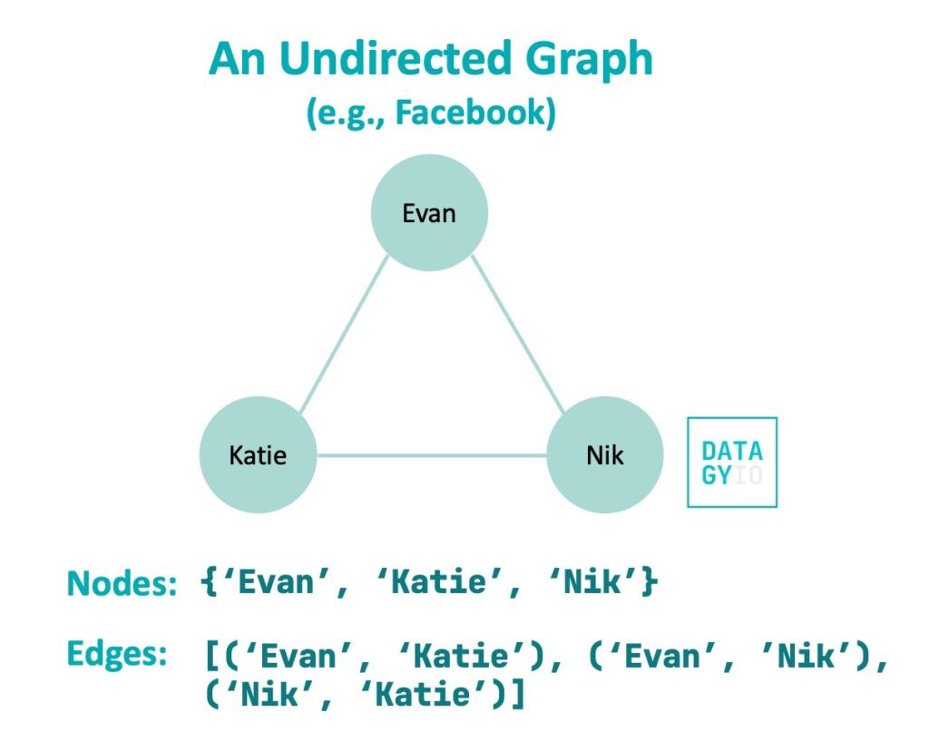
This is an example of an undirected graph. This means that the relationship between two nodes occurs in both directions. Because of this, a sample edge may connect Evan and Katie. This edge would be represented by {'Evan', 'Katie'}. Note that we used a set to represent this. In this case, the relationship goes both ways.

Now let’s take a look at another example. Imagine that we’re modeling relationships in X (formerly Twitter). Because someone can follow someone without the other person following them back, we can end up with a relationship like the one shown below.

This is an example of a directed graph. Notice that the edges here are represented as arrows. In this case, Nik and Katie follow one another, but the same isn’t true for the others. Evan follows Katie (but not the other way around). Similarly, Nik follows Evan, but not the other way around.

In this case, while our nodes remain the same as {'Nik', 'Evan', 'Katie'}, our edge list now has a different meaning. In fact, it’s easier to use a list of tuples to represent this now, where the first value is the starting node and the second is the end node. This would look like this: [('Nik', 'Katie'), ('Katie', 'Nik'), ('Evan', 'Katie'), ('Nik', 'Evan')].

Let’s now dive a little further into the different types of graphs and how they can be represented in Python.

Want to learn how to traverse these graphs? Check out my in-depth guides on breadth-first search in Python and depth-first search in Python.

Understanding Graph Data Structure Representations

In this tutorial, we’ll explore three of the most fundamental ways in which to represent graphs in Python. We’ll also explore the benefits and drawbacks of each of these representations. Later, we’ll dive into how to implement these for different types of graphs and how to create these in Python.

One of the ways you have already seen is called an edge list. The edge list lists our each of the node-pair relationships in a graph. The list can include additional information, such as weights, as you’ll see later on in this tutorial.

In Python, edge lists are often represented as lists of tuples. Let’s take a look at an example:

# A sample edge list
edge_list = [('A', 'B'), ('B', 'C'), ('B', 'D'), ('C', 'E'), ('D', 'E'), ('E', 'F')]

In the code block above, we can see a sample edge list. In this case, each pair represents an unweighted relationship (since no weight is given) between two nodes. In many cases, edge lists for undirected graphs omit the reverse pair (so ('A', 'B') represents both sides of the relationship, for example).

Another common graph representation is the adjacency matrix. Adjacency matrices are often represented as lists of lists, where each list represents a node. The list’s items represent whether an edge exists between the node and another node.

Let’s take a look at what this may look like:

# A sample adjacency matrix
[[0, 1, 0, 0, 0, 0],
 [1, 0, 1, 1, 0, 0],
 [0, 1, 0, 0, 1, 0],
 [0, 1, 0, 0, 1, 0],
 [0, 0, 1, 1, 0, 1],
 [0, 0, 0, 0, 1, 0]]

In the example above, we can see all the node’s connections. For example, node 'A' comes first. We can see that it has an edge only with node 'B'. This is represented by 1, where all other nodes are 0.

One of the key benefits of an adjacency matrix over an edge list is that we can immediately see any node’s neighbors, without needing to iterate over the list.

However, adjacency matrices are often very sparse, especially for graphs with few edges. Because of this, the preferred method is the adjacency list.

An adjacency list is a hash map that maps each node to a list of neighbors. This combines the benefits of both the edge list and the adjacency matrix, by providing a contained structure that allows you to easily see a node’s neighbors.

In Python, adjacency lists are often represented as dictionaries. Each key is the node label and the value is either a set or a list of neighbors. Let’s take a look at an example:

# A sample adjacency list
{
    'A': ['B'],
    'B': ['A', 'C', 'D'],
    'C': ['B', 'E'],
    'D': ['B', 'E'],
    'E': ['C', 'D', 'F'],
    'F': ['E']
}

Let’s quickly summarize the three main structures for different graph types:

Aspect	Undirected Graph	Directed Graph	Weighted Graph
Edge Representation	Edges are represented as (A, B) or (B, A) to denote the lack of direction.	Edges are represented as (A, B) to indicate direction from A to B.	Edges are represented as (A, B, weight) to include edge weights.
Edge List Structure	List of tuples: [(0, 1), (0, 2), ...]	List of tuples: [(0, 1), (0, 2), ...]	List of tuples: [(0, 1, 5), (0, 2, 3), ...] (source, destination, weight)
Adjacency Representation	Adjacency lists or matrices hold connections between nodes. Edges are bidirectional.	Adjacency lists or matrices hold connections between nodes, specifying direction.	Adjacency lists or matrices hold connections with associated edge weights.
Node Connectivity	Nodes are connected bidirectionally.	Edges have a specific direction from one node to another.	Edges have weights representing the cost or value associated.
Example	[(0, 1), (0, 2), (1, 2), ...]	Edges are represented as (A, B) to indicate the direction from A to B.	[(0, 1, 5), (0, 2, 3), (1, 2, 2), ...] (source, destination, weight)

Now that you have a good understanding of how graphs can be represented, let’s dive into some more practical examples by exploring different graph types.

Understanding Undirected Graph Data Structures

As we saw earlier, an undirected graph has edges that connect nodes without specifying direction, because the edges are bidirectional. In the edge list representation an edge connecting ('A', 'B') is the same as that connecting ('B', 'A').

Let’s take a look at a more complete example of what this can look like. We’ll use nodes labeled A through F for this and look at different ways in which this graph can be represented.

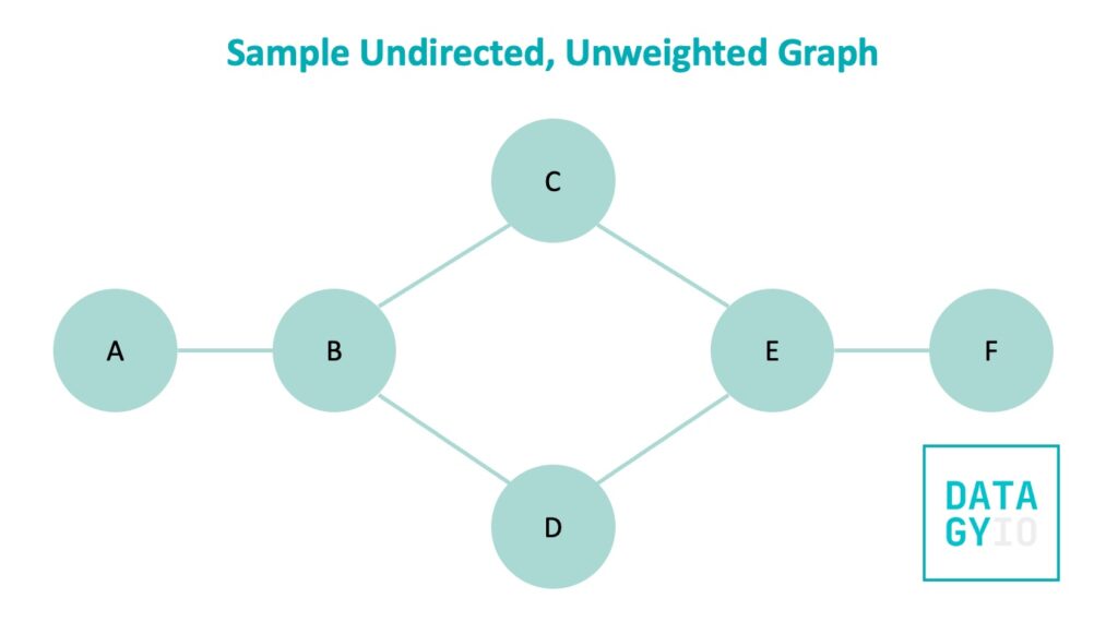
We can see that in the image above all nodes are connected by lines without heads. This indicates that the graph is undirected and that the relationship is bidirectional. As an edge list, this graph would be represented as shown below:

# Edge list for an undirected graph
edge_list = [('A', 'B'), ('B', 'C'), ('B', 'D'), ('C', 'E'), ('D', 'E'), ('E', 'F')]

In this case, it’s important to note that the graph is undirected. Without this knowledge, half the relationships would be lost. Because of this, it can sometimes be helpful to be more explicit and list out all possible relationships, as shown below:

# Being explicit in undirect relationships
undirected = [('A', 'B'), ('B', 'A'), ('B', 'C'), ('C', 'B'), ('B', 'D'), ('D', 'B'), ('C', 'E'), ('E', 'C'), ('D', 'E'), ('E', 'D'), ('E', 'F'), ('F', 'E')]

In the code block above, we’re repeating each relationship for each node-pair relationship. While this is more explicit, it’s also redundant.

One problem with edge lists is that if we want to see any node’s neighbors, we have to iterate over the entire list. Because of this, there are different representations that we can use.

Adjacency Matrix for Undirected, Unweighted Graphs

Another common way to represent graphs is to use an adjacency matrix. In Python, these are lists of lists that store the corresponding relationship for each node. For example, our graph has seven nodes. Because of this, the adjacency matrix will have seven lists, each with seven values.

Take a look at the image below to see what our adjacency matrix for our undirected, unweighted graph looks like:

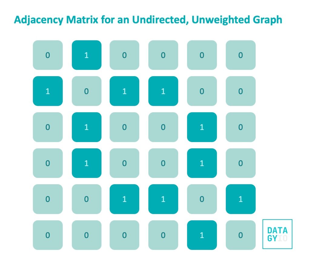
In the image above, we can see our matrix of seven rows and seven values each. The first row shows all the relationships that node 'A' has. We can see that it only connects to the second node, 'B'. In this case, edges are labelled at 1 and non-existent edges are labelled as 0.

One unique property of an adjacency matrix for undirected graphs is that they are symmetrical! If we look along the diagonal, we can see that the values are mirrored.

Let’s take a look at how we can write a function to accept an edge list and return an adjacency matrix in Python:

# Creating an adjacency matrix in Python
def edge_list_to_adjacency_matrix(edge_list, directed=False):
    nodes = set()
    for edge in edge_list:
        nodes.add(edge[0])
        nodes.add(edge[1])

    nodes = sorted(list(nodes))
    num_nodes = len(nodes)
    adjacency_matrix = [[0] * num_nodes for _ in range(num_nodes)]

    for edge in edge_list:
        index_1 = nodes.index(edge[0])
        index_2 = nodes.index(edge[1])
        adjacency_matrix[index_1][index_2] = 1
        if not directed:
            adjacency_matrix[index_2][index_1] = 1

    return adjacency_matrix

In the code block above, we created a function that creates an adjacency matrix out of an edge list. The function creates a set out of our nodes and then sorts that set. We then create a matrix that creates a list of lists of 0s for each node in the graph.

The function then iterates over the edges and finds the indices for each node. It adds 1 for each edge it finds. By default, the function assumes an undirected graph; if this is the case, it also adds a 1 for each reverse pair.

When we run the function on a sample edge list, we get the following code back:

# Creating an adjacency matrix with our function
edge_list = [('A', 'B'), ('B', 'C'), ('B', 'D'), ('C', 'E'), ('D', 'E'), ('E', 'F')]
adj_matrix = edge_list_to_adjacency_matrix(edge_list)
print(adj_matrix)

# Returns:
# [[0, 1, 0, 0, 0, 0],
#  [1, 0, 1, 1, 0, 0],
#  [0, 1, 0, 0, 1, 0],
#  [0, 1, 0, 0, 1, 0],
#  [0, 0, 1, 1, 0, 1],
#  [0, 0, 0, 0, 1, 0]]

Now let’s take a look at adjacency lists for undirected, unweighted graphs.

Adjacency List for Undirected, Unweighted Graphs

For graphs that don’t have many edges, adjacency matrices can become very sparse. Because of this, we can use one of the most common graph representations, the adjacency list. The adjacency list combines the benefits of both the edge list and the adjacency matrix by creating a hash map of nodes and their neighbors.

Let’s take a look at what an adjacency list would look like for an undirected, unweighted graph:

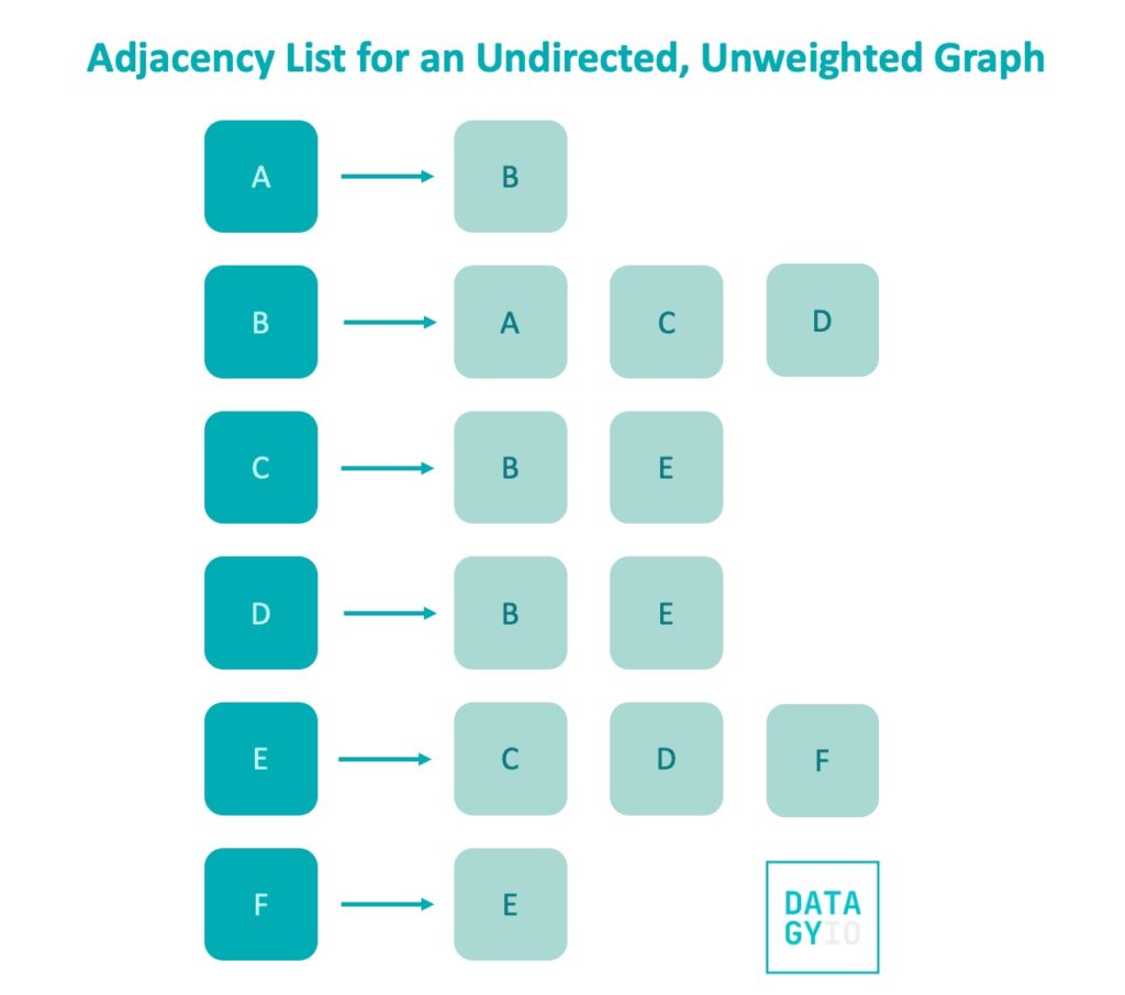
In Python, we would represent this using a dictionary. Let’s take a look at how we can create a function that accepts an edge list and returns an adjacency list:

# Defining a function to create an adjacency list
def edge_list_to_adjacency_list(edge_list, directed=False):
    adjacency_list = {}
    
    for edge in edge_list:
        node_1, node_2 = edge
        
        if node_1 not in adjacency_list:
            adjacency_list[node_1] = []
        adjacency_list[node_1].append(node_2)

        if not directed:
            if node_2 not in adjacency_list:
                adjacency_list[node_2] = []
            adjacency_list[node_2].append(node_1)

    return adjacency_list

This function is a bit simpler than our previous function. We accept both an edge list and whether our graph is directed or not. We then create a dictionary to hold our adjacency list. The iterate over each edge in our list. We check if the starting node exists in our dictionary – if it doesn’t we create it with an empty list. We then append the second node to that list.

Similarly, if the graph is not directed, we do the same thing for the inverse relationship.

Let’s take a look at what this looks like for a sample edge list:

# Using our adjacency list function
edge_list = [('A', 'B'), ('B', 'C'), ('B', 'D'), ('C', 'E'), ('D', 'E'), ('E', 'F')]
adj_list = edge_list_to_adjacency_list(edge_list)
print(adj_list)

# Returns:
# {'A': ['B'],
#  'B': ['A', 'C', 'D'],
#  'C': ['B', 'E'],
#  'D': ['B', 'E'],
#  'E': ['C', 'D', 'F'],
#  'F': ['E']}

Now that you have a strong understanding of the three representations of unweighted, undirected graphs, let’s take a look at directed graphs in Python.

Understanding Directed Graph Data Structures

Directed graphs, also known as digraphs, are networks where edges between nodes have a defined direction. Unlike undirected graphs, edges in directed graphs are unidirectional, representing a directed relationship from one node (the source) to another node (the target or destination).

Directed graphs can be helpful when modeling one-way relationships, such as one-way streets, task dependencies in project management, or social media followings.

Let’s take a look at what one of these graphs may look like:

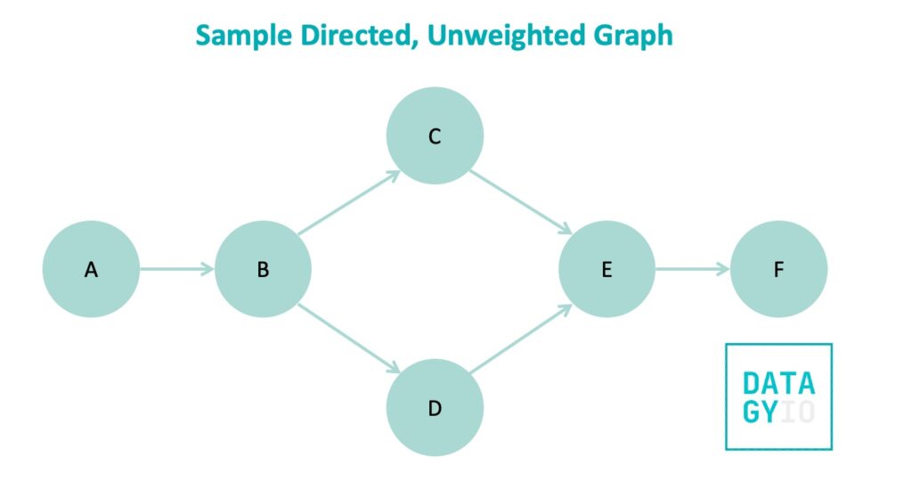
We can see that this graph looks very similar to the one that we saw before. However, each edge has a direction on it. In this example, each edge is one-directional. However, directed graphs can also have bi-directional edges.

In this case, we can use an adjacency matrix to represent this graph as well. This is shown in the image below:

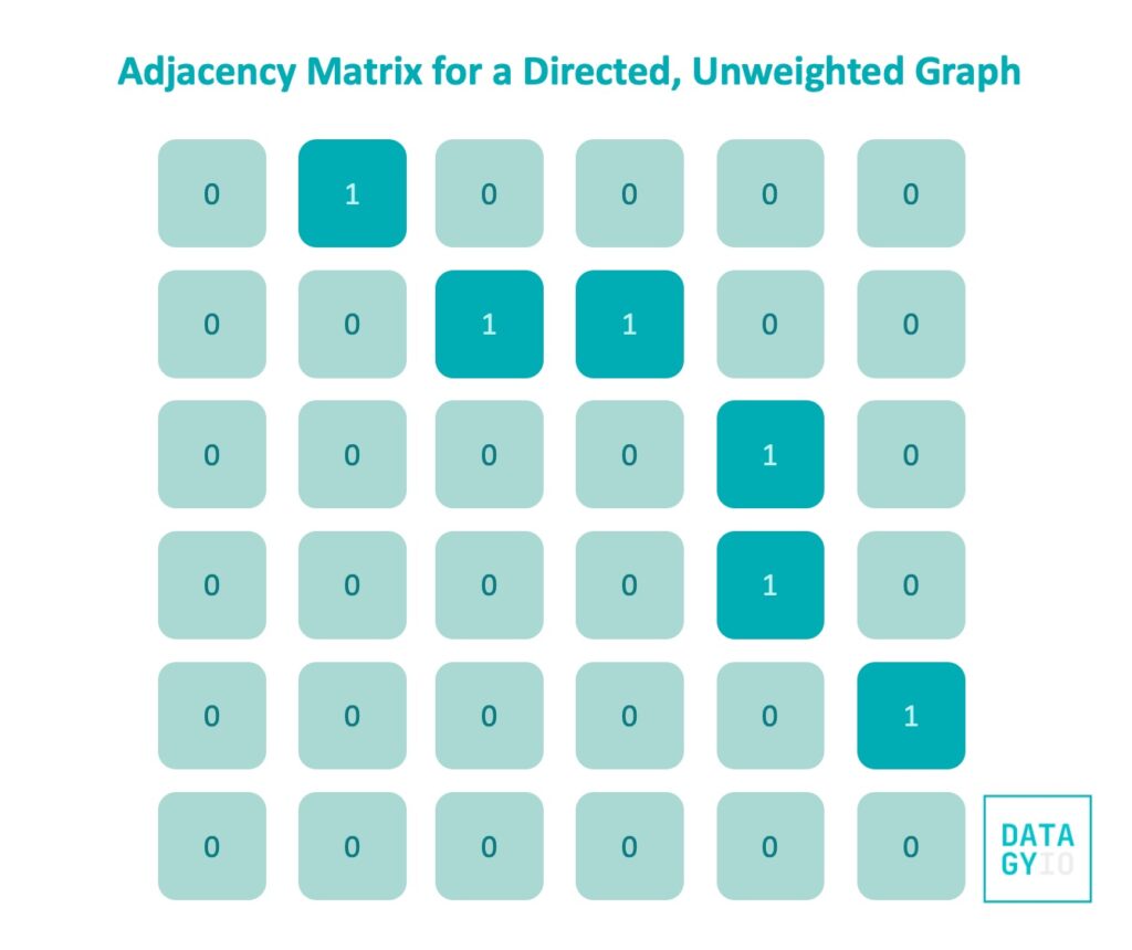
The function that we developed earlier is already built around the concept of directed graphs. In order to use it, we simply need to indicate that the graph is directed. Let’s take a look at what this looks like:

# Converting an Edge List to a Directed Adjacency Matrix
def edge_list_to_adjacency_list(edge_list, directed=False):
    adjacency_list = {}
    
    for edge in edge_list:
        node_1, node_2 = edge
        
        if node_1 not in adjacency_list:
            adjacency_list[node_1] = []
        adjacency_list[node_1].append(node_2)

        if not directed:
            if node_2 not in adjacency_list:
                adjacency_list[node_2] = []
            adjacency_list[node_2].append(node_1)

    return adjacency_list

adj_matrix = edge_list_to_adjacency_matrix(edge_list, directed=True)
print(adj_matrix)

# Returns:
# [[0, 1, 0, 0, 0, 0],
#  [0, 0, 1, 1, 0, 0],
#  [0, 0, 0, 0, 1, 0],
#  [0, 0, 0, 0, 1, 0],
#  [0, 0, 0, 0, 0, 1],
#  [0, 0, 0, 0, 0, 0]]

The only change that we made was in calling the function: we modified the default argument of directed=False to True. This meant that the bi-directional pair was not added to our matrix.

Similarly, we can use adjacency lists to represent directed graphs. Let’s take a look at what this would look like:

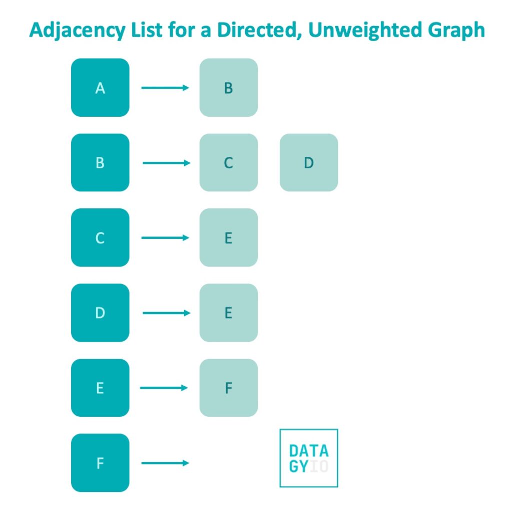
In the image above, each dictionary key is still represented by the starting node and the list of values is represented by its neighbors.

Similarly, the function we previously created allows us to pass in that we’re working with a directed graph. Let’s see what this looks like:

# Creating an adjacency list from an edge list
def edge_list_to_adjacency_list(edge_list, directed=False):
    adjacency_list = {}
    
    for edge in edge_list:
        node_1, node_2 = edge
        
        if node_1 not in adjacency_list:
            adjacency_list[node_1] = []
        adjacency_list[node_1].append(node_2)

        if not directed:
            if node_2 not in adjacency_list:
                adjacency_list[node_2] = []
            adjacency_list[node_2].append(node_1)

    return adjacency_list

# Using our adjacency list function
edge_list = [('A', 'B'), ('B', 'C'), ('B', 'D'), ('C', 'E'), ('D', 'E'), ('E', 'F')]
adj_list = edge_list_to_adjacency_list(edge_list, directed=True)
print(adj_list)

# Returns: {'A': ['B'], 'B': ['C', 'D'], 'C': ['E'], 'D': ['E'], 'E': ['F']}

Similar to our previous example, we only modified the default argument of directed= to True. This allowed us to create an adjacency list for a directed graph.

Now that we’ve covered unweighted graphs, let’s dive into weighted graphs, which add additional information to our graph.

Understanding Weighted Graph Data Structures

Weighted directed graphs expand upon directed graphs by incorporating edge weights, assigning a value or cost to each directed edge between nodes. In this graph type, edges not only depict directional relationships but also carry additional information in the form of weights, indicating the strength, distance, cost, or any other relevant metric associated with the connection from one node to another.

These weights add an extra layer of complexity and significance, allowing the representation of various scenarios where the intensity or cost of relationships matters. Weighted directed graphs find applications in diverse fields such as logistics, transportation networks, telecommunications, and biology, where the weights might represent distances between locations, communication costs, strengths of interactions, or genetic similarities.

Let’s use our previous example graph and add some weights to it:

We can represent these graphs as adjacency matrices as well. In this case, rather than using the default value of 1, we represent each node by the weight that it has. Take a look at the image below for how this representation works:

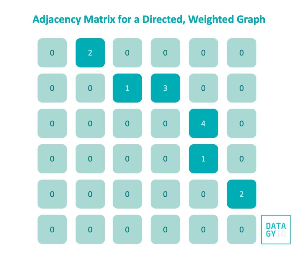
To convert an edge list to an adjacency matrix using Python, we only have to make a small adjustment to our function. Let’s take a look at what this looks like:

# Creating a function to convert a weighted edge list into an adjacency matrix
def edge_list_to_adjacency_matrix(edge_list, directed=False, weighted=False):
    nodes = set()
    for edge in edge_list:
        nodes.add(edge[0])
        nodes.add(edge[1])

    nodes = sorted(list(nodes))
    num_nodes = len(nodes)
    adjacency_matrix = [[0] * num_nodes for _ in range(num_nodes)]

    for edge in edge_list:
        index_1 = nodes.index(edge[0])
        index_2 = nodes.index(edge[1])
        weight = edge[2] if weighted else 1
        adjacency_matrix[index_1][index_2] = weight
        if not directed:
            adjacency_matrix[index_2][index_1] = weight

    return adjacency_matrix

weighted = [('A', 'B', 2), ('B', 'C', 1), ('B', 'D', 3), ('C', 'E', 4), ('D', 'E', 1), ('E', 'F', 2)]
adj_matrix = edge_list_to_adjacency_matrix(weighted, directed=True, weighted=True)
print(adj_matrix)

# Returns:
# [[0, 2, 0, 0, 0, 0],
#  [0, 0, 1, 3, 0, 0],
#  [0, 0, 0, 0, 4, 0],
#  [0, 0, 0, 0, 1, 0],
#  [0, 0, 0, 0, 0, 2],
#  [0, 0, 0, 0, 0, 0]]

In this case, we added a second optional parameter that indicates whether a graph is weighted or not. We use the ternary operator to assign the weight if the graph is weighted, otherwise use the default value of 1.

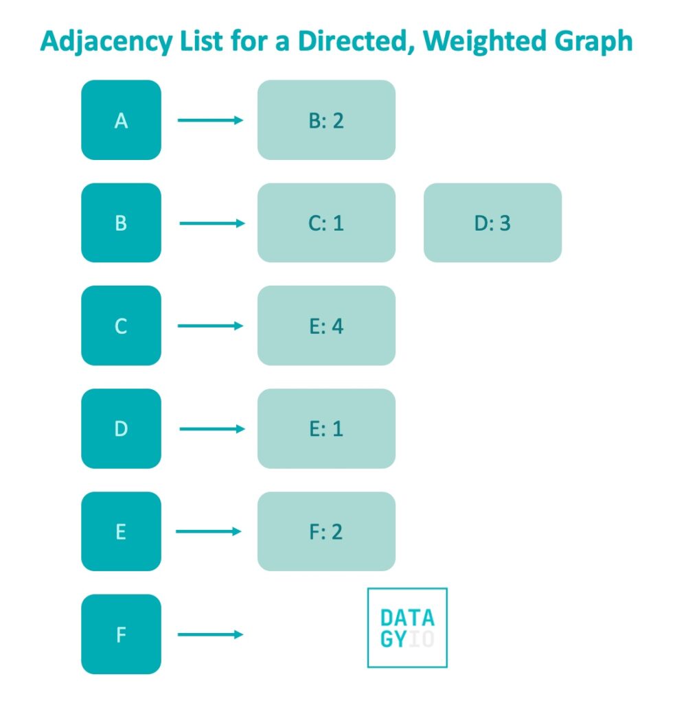
In an adjacency list, the keys continue to represent the nodes of the graph. The values are now lists of tuples that contain the end node and the weight for that relationship. Take a look at the image below to see what this looks like:

We can make small modifications to our earlier function to allow for weighted graphs. Let’s see what this looks like:

# Creating an adjacency list from an edge list
def edge_list_to_adjacency_list(edge_list, directed=False, weighted=False):
    adjacency_list = {}
    
    for edge in edge_list:
        node_1 = edge[0]
        node_2 = edge[1]
        if weighted:
            weight = edge[2]
        
        if node_1 not in adjacency_list:
            adjacency_list[node_1] = []
        if weighted:
            adjacency_list[node_1].append((node_2, weight))
        else:
            adjacency_list[node_1].append(node_2)

        if not directed:
            if node_2 not in adjacency_list:
                adjacency_list[node_2] = []
            if weighted:
                adjacency_list[node_2].append((node_1, weight))
            else:
                adjacency_list[node_2].append(node_1)

    return adjacency_list

adj_list = edge_list_to_adjacency_list(weighted, directed=True, weighted=True)
print(adj_list)

# Returns:
# {'A': [('B', 2)],
#  'B': [('C', 1), ('D', 3)],
#  'C': [('E', 4)],
#  'D': [('E', 1)],
#  'E': [('F', 2)]}

In the code block above, we modified our function to accept a third argument, indicating whether the graph is weighted or not. We then added a number of if-else statements to get the weight from our edge list if the edge list has weights in it.

We can see that the function returns a dictionary that contains lists of tuples, which represent the end node and the weight of the relationship.

Conclusion

Understanding how to represent graphs in Python is essential for anyone working with complex relationships and networks. In this tutorial, we explored three fundamental ways to represent graphs: edge lists, adjacency matrices, and adjacency lists. Each method has its strengths and trade-offs, catering to different scenarios and preferences.

We began by dissecting what graphs, nodes, and edges are, showcasing examples of undirected and directed graphs. From there, we delved into the details of each representation method:

• Edge Lists: Simple and intuitive, representing relationships between nodes as tuples.
• Adjacency Matrices: Efficient for determining connections between nodes but can become sparse in large, sparse graphs.
• Adjacency Lists: Efficient for sparse graphs, offering quick access to a node’s neighbors.

We explored these representations for different graph types, including undirected, directed, and weighted graphs. For each type, we demonstrated how to convert between representations using Python functions.

Understanding these representations equips you to handle diverse scenarios, from modeling social networks to logistical networks, project management, and more. Graphs are a powerful tool for modeling relationships, and grasping their representations in Python empowers you to analyze and work with complex interconnected data effectively.

The official Python documentation also has useful information on building graphs in Python.