Dijkstra’s Algorithm (Shortest Path) in Python

In this tutorial, you’ll learn how to implement Dijkstra’s Algorithm in Python to find the shortest path from a starting node to every node in a graph. The algorithm allows you to easily and elegantly calculate the distances, ensuring that you find the shortest path.

By the end of this tutorial, you’ll have learned the following:

• The intuition behind Dijkstra’s algorithm using pseudocode
• How to use Dijkstra’s algorithm to find the shortest path
• How to implement Dijkstra’s algorithm in Python

Understanding Dijkstra’s Algorithm to Find the Shortest Path

The best way to understand Dijkstra’s Algorithm for the shortest path is to look at an example. We’ll use a fairly simple graph for this tutorial, in order to make following along a little bit easier.

Take a look at the graph below. It’s a weighted, undirected graph, meaning that each edge connects bi-directionally and each edge has an associated weight.

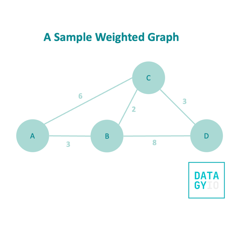
In this example walkthrough, we’ll be looking for the shortest path connect any node to node 'A'. To clarify this further, we’ll want to what the shortest path to nodes ['B', 'C', 'D'] are. Because our edges are weighted, sometimes taking multiple steps will actually be faster!

In order to implement Dijkstra’s Algorithm, we’ll want to keep track of a number of different pieces. In particular, we’ll need to track:

1. The currently known shortest distances from node A to any node,
2. Which nodes we have visited so far
3. Which previous node (or vertex) resulted in the shortest path

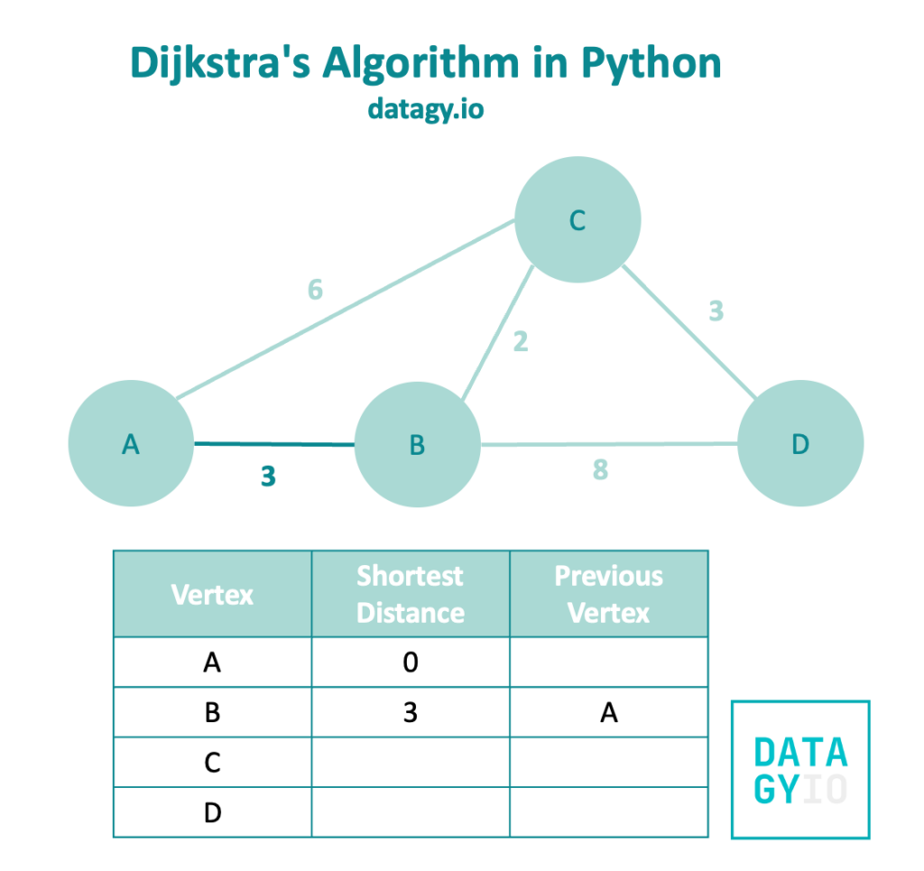
Let’s set up our example graph with a table to track all of this information, as shown in the image below:

You can see that we have already labeled the distance from 'A' to itself. In this case, that weight is 0.

Dijkstra’s Algorithm follows a breadth-first search, favoring edges of smaller weights. When we look at our example graph, we can see that 'A' has two neighbors, ['B', 'C']. Because 'B' has a smaller weight, we look at this node first.

We can see that because we hadn’t visited node 'B' yet, this edge represents the shortest path! So we add it to our table and include vertex 'A' as the previously visited vertex.

We then follow our breadth-first search and visit node 'A'‘s other neighbor, node 'C'.

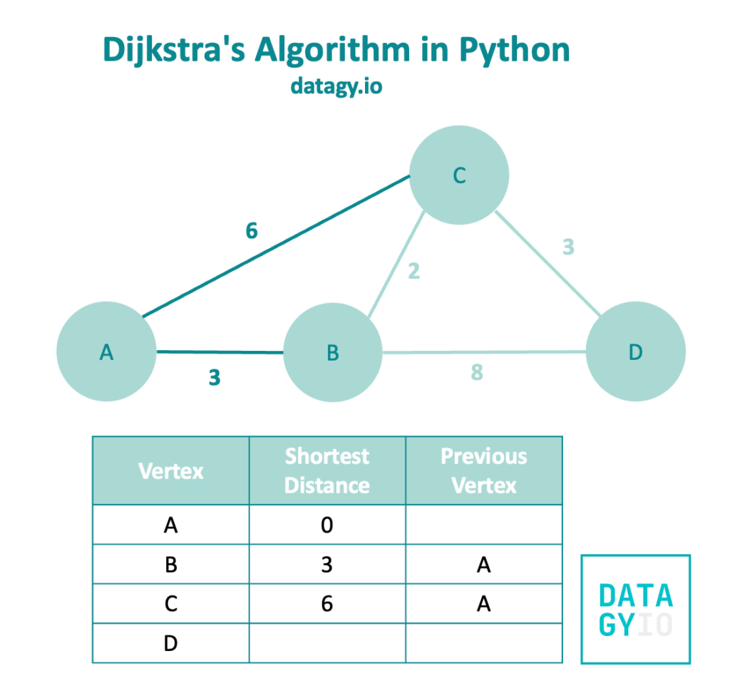
Because we haven’t visited node 'C' yet, we add its edge’s weight to the shortest distance. Similarly, we make note that we visited this node from 'A'.

We then follow our breadth-first search further and take a look at the neighbors of node 'B'. In this case, these neighbors are ['C', 'D']. Node 'C' has a smaller weight, so we visit this first.

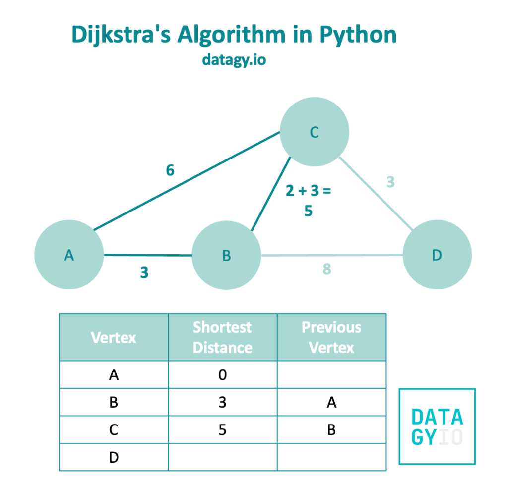
Rather than including only the weight of 2, we actually add it to the original distance of 3. This is because we’re interested in how much distance 'C' is from 'A', not from 'B'. In this case, this distance is 5.

Because 5 is less than our original distance of 8, we replace this value in the table and modify the previous vertex. This is our first example where visiting a node via another node is faster than visiting it directly!

Now, we need to take a look at visiting node 'D' from node 'B'. We’ll follow a similar process and add the original distance (3) to the weight of 8.

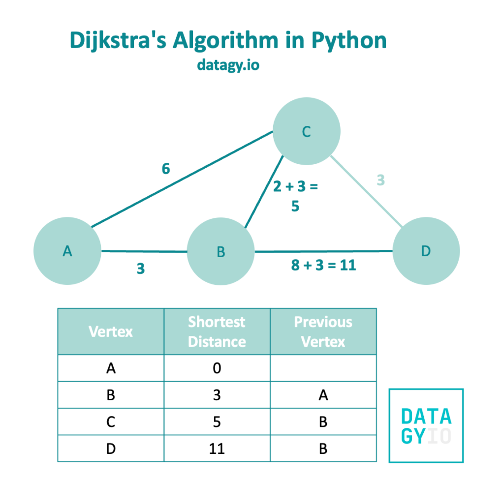
We can see that this gives us a weight of 11 and a previous vertex of 'B'.

Because 'B' has no more unvisited neighbors, we then look at the neighbors of node 'C'. The only unvisited neighbor is node 'D'.

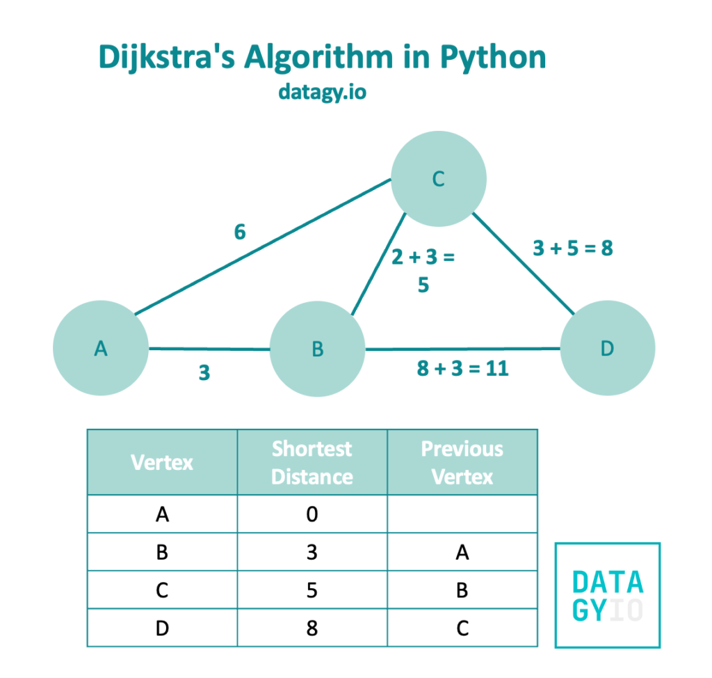
We’ll add the original shortest distance to get to node 'C' (5) to the weight (3) and get a value of 8 back. Because this value is less than 11 (our previous shortest distance), we replace this value in our table.

Now that you’ve built a strong intuition for how Dijkstra’s Algorithm works, let’s take a look at how we can implement it using pseudo-code!

Pseudocode for Dijkstra’s Algorithm

In the previous example, we implement Dijkstra’s Algorithm visually, using a breadth-first approach. What can make the process even better is to use a “best-first approach”. For this, we implement a min-heap. This allows us to use a heap, rather than a queue for our data. What this means is that the heap will pick the value with the lowest weight to visit next, rather than the subsequent item.

Let’s see what this looks like in pseudo-code:

function Dijkstra(graph, start):
    distances = {node: infinity for node in graph}
    distances[start] = 0
    priority_queue = [(0, start)]

    while priority_queue is not empty:
        current_distance, current_node = pop smallest element from priority_queue

        if current_distance > distances[current_node]:
            continue

        for neighbor, weight in neighbors of current_node in graph:
            distance = current_distance + weight

            if distance < distances[neighbor]:
                distances[neighbor] = distance
                push (distance, neighbor) to priority_queue

    return distances

Let’s break down what our pseudo-code is doing:

1. We define a function that accepts our graph and starting vertex
2. When then create a dictionary that holds each node as the key and the value infinite for each distance
3. When then set the distance from the starting node to itself to 0
4. We add this to our priority queue
5. We then use a while loop to continue while our priority queue is not empty and grab the smallest item from the queue
6. If the current distance is larger than the distance we have recorded in our dictionary, we continue to the next iteration
7. Otherwise, we loop over each neighbor of the current node. We grab its distance and weight and add them together. If the distance is smaller than the smallest known distance, we update the dictionary and push these values to the heap

Now that you have a strong understanding of how the code should work, let’s begin implementing it in Python!

Implementing Dijkstra’s Algorithm in Python

In this section, we’ll explore how to implement Dijkstra’s Algorithm in Python. Our first step will be to convert our graph visual into an edge list. Remember, our graph looks like this:

We can create an edge list out of this by using a list of tuples, as shown below:

# Converting our graph to an edge list
edge_list = [('A', 'B', 3), ('A', 'C', 8), ('B', 'C', 2), ('B', 'E', 5), ('C', 'D', 1), ('C', 'E', 6), ('D', 'E', 2), ('D', 'F', 3), ('E', 'F', 5)]

To make this easier to work with, we can change the representation of the edge list to an adjacency list. Each key will be a node and the value will be a dictionary that contains the node’s neighbors and their weights. For this, we can use a custom function:

# Converting our graph to an adjacency list
def edge_list_to_adjacency_list(edge_list):
    adj_list = {}
    for (src, dest, weight) in edge_list:
        if src not in adj_list:
            adj_list[src] = {}
        if dest not in adj_list:
            adj_list[dest] = {}
        
        adj_list[src][dest] = weight
        adj_list[dest][src] = weight

    return adj_list

adj_list = edge_list_to_adjacency_list(edge_list)
print(adj_list)

# Returns:
# {
#     'A': {'B': 3, 'C': 8},
#     'B': {'A': 3, 'C': 2, 'E': 5},
#     'C': {'A': 8, 'B': 2, 'D': 1, 'E': 6},
#     'E': {'B': 5, 'C': 6, 'D': 2, 'F': 5},
#     'D': {'C': 1, 'E': 2, 'F': 3},
#     'F': {'D': 3, 'E': 5}
#  }

Now that we have an adjacency list, let’s begin by implementing Dijkstra’s algorithm:

# Implementing Dijkstra's Algorithm in Python
import heapq

def dijkstra(adj_list, start):
    distances = {node: float('inf') for node in adj_list}
    distances[start] = 0

    # Priority queue to track nodes and current shortest distance
    priority_queue = [(0, start)]

    while priority_queue:
        # Pop the node with the smallest distance from the priority queue
        current_distance, current_node = heapq.heappop(priority_queue)

        # Skip if a shorter distance to current_node is already found
        if current_distance > distances[current_node]:
            continue

        # Explore neighbors and update distances if a shorter path is found
        for neighbor, weight in adj_list[current_node].items():
            distance = current_distance + weight

            # If shorter path to neighbor is found, update distance and push to queue
            if distance < distances[neighbor]:
                distances[neighbor] = distance
                heapq.heappush(priority_queue, (distance, neighbor))

    return distances

Let’s take a look at what this code is doing. If you already understand the pseudo-code, this will translate nicely.

The dijkstra function takes in an adjacency list representation of the graph and a starting node as arguments. Initially, it sets all distances to infinity except for the starting node, which is set to 0.

A priority queue (priority_queue) is created to keep track of nodes along with their current shortest distances. The algorithm uses this queue to process nodes based on their distances from the starting node.

The main loop of the algorithm continues as long as there are nodes in the priority queue. It retrieves the node with the smallest known distance (current_distance) from the queue using heapq.heappop(priority_queue).

Within the loop, the algorithm checks whether a shorter distance to the current node (current_node) has already been found. If so, it skips further exploration of that node to prioritize more efficient paths.

For each neighbor of the current node, the algorithm calculates a potential shorter distance by adding the edge weight between the nodes to the current distance. If this new distance is shorter than the previously recorded distance to the neighbor node, the algorithm updates the distance and pushes the updated distance and node pair into the priority queue for further exploration.

This process continues until the priority queue becomes empty, ensuring that the algorithm explores nodes, updates distances, and identifies the shortest paths from the starting node to all reachable nodes in the graph.

Finally, the function returns a dictionary containing the shortest distances from the starting node to all other nodes in the graph.

Conclusion

In this comprehensive tutorial, we delved into understanding and implementing Dijkstra’s Algorithm in Python for finding the shortest path from a starting node to all other nodes in a graph. By following along, you’ve gained insights into how this algorithm elegantly calculates distances, ensuring the discovery of the shortest paths within a graph.

To learn more about Dijkstra’s Algorithm, check out this page on it.