Connected Components in Graphs Algorithm in Python

Graphs are powerful models that span many different domains, such as infrastructure, GPS navigation, and social networks. Within these graphs are interconnected regions, which are known as connected components. Understanding these components is pivotal in understanding relationships and identifying isolated clusters. In this tutorial, you’ll learn how to count the number of components in a given graph using Python.

By the end of this tutorial, you’ll have learned the following:

• How to understand components within a graph
• How to write an algorithm in Python to count the number of components
• How to use NetworkX to count the number of components

Understanding Graph Components

Graphs, comprised of nodes (vertices) and edges connecting these nodes, serve as a fundamental abstraction for modeling relationships between various entities. They come in various types—directed and undirected—each representing unique connectivity patterns.

I have put together a complete tutorial on how graphs can be represented in Python, covering unweighted and weighted, undirected and directed graphs.

A component in graph theory refers to a collection of nodes within a graph where each of the nodes is either directly or indirectly connected to every other node in that subset.

By knowing how to count components within a graph, you can understand its complexity, connectivity, and the relationships between different subsets of nodes.

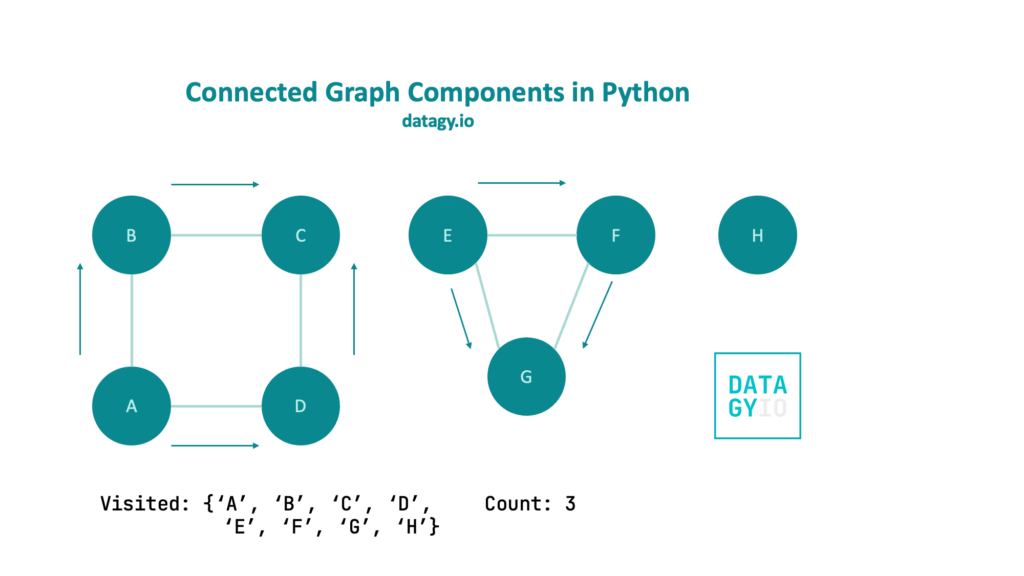
Let’s take a look at the following graph, with three different components:

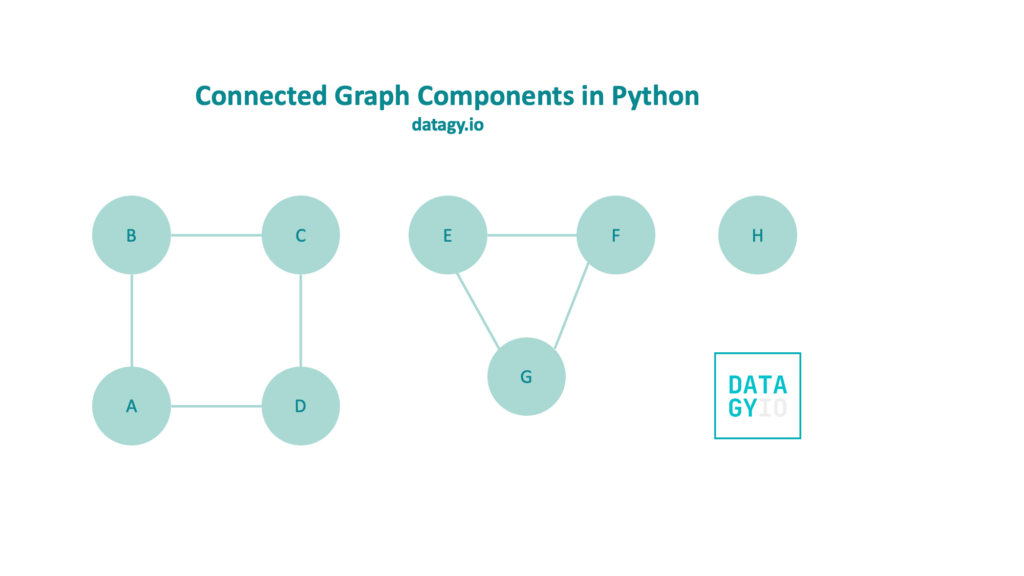
Intuitively, we can see that there are separate components in our graph. However, it can be beneficial to come up with some programmatic way to count the number of components. Let’s take a look at some visuals to guide us through this:

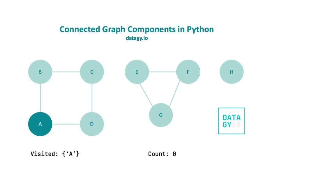
In the image above, we find a starting node. In this case, we’re using 'A', since it’s the first node in our adjacency list. We instantiate two variables:

1. visited, which is a set that stores our visited nodes
2. count, which counts how many components exist in our graph

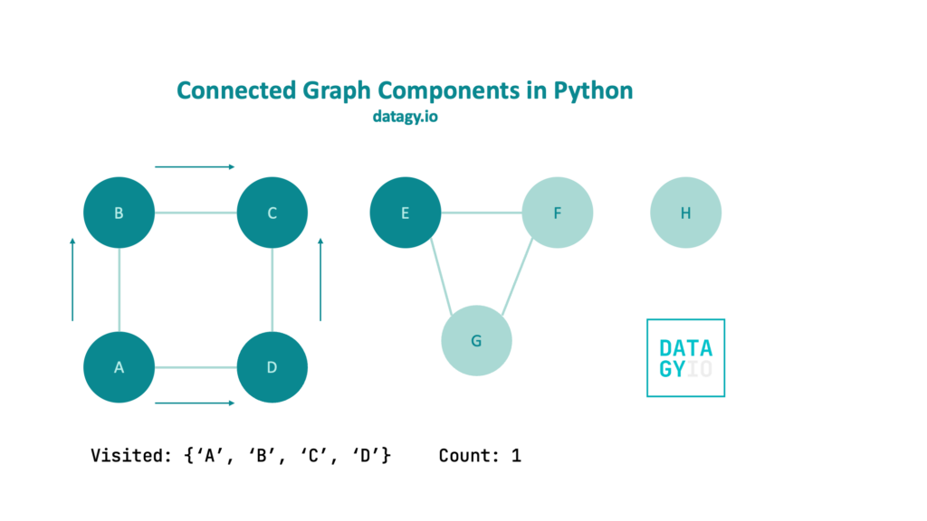
We first iterate explore all of the nodes neighbors. In this case, we’re using a breadth-first approach, but you could easily accomplish this with a depth-first search as well. Once our breadth-first search is complete and we have added all of the node’s neighbors to our visited set, we increment our count by 1.

Then, we move on to the next node in our graph. For any node that hasn’t been visited, we run BFS. In this case, we cycle through the nodes A through D before moving on to our next component as shown below:

We repeat our breadth-first search through this component and increment our count by 1.

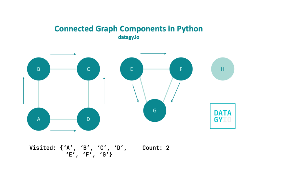
Finally, we have a lone node, which doesn’t have neighbors, so we simply increment our count by 1.

This might look like there’s a lot of required code, but it’s actually quite simple. Let’s build some pseudo-code in the following section to nuance this out.

Counting Graph Components in Python Pseudo-Code

In this section, we’ll create some pseudo-code to model an algorithm to count components in a graph. Understanding the pseudo-code will allow you to have a strong understanding of how to write the code:

count_components(graph):
    visited = empty set
    components = 0
    
    for each node in graph:
        if node not in visited:
            queue = empty queue
            queue.enqueue(node)
            visited.add(node)
            
            while queue is not empty:
                current_node = queue.dequeue()
                for each neighbor in graph[current_node]:
                    if neighbor not in visited:
                        visited.add(neighbor)
                        queue.enqueue(neighbor)
            
            components += 1
    
    return components

Let’s break down what this code is down:

1. We first instantiate a new set to track visited nodes and set the count of components to 0
2. We then iterate through each node in the graph. First, we check if the node has not been visited. If it hasn’t, we create an empty queue and add it to the queue.
3. From there, we add the node to our visited set.
4. While our queue is not empty, we then iterate over all of the neighbors of that node and add them to our visited set.
5. Finally, when all neighbors have been visited, we add 1 to our component count.
6. We then move to the next node (which will part of our next component)

Now that you have a good understanding of how the algorithm should work, let’s implement this in Python!

Counting Graph Components in Python Algorithm

In this section, we’ll explore how to implement a counting graph components algorithm in Python. This section will assume that you’re familiar with either of the following algorithms:

1. Depth-first search or
2. Breadth-first search

For this tutorial, we’ll focus on using a breadth-first approach. However, the algorithm will work in the same way for a depth-first approach as well.

Let’s start by defining our function to count components:

def count_components(graph):
    visited = set()
    components = 0
    for node in graph:
        if node not in visited:
            bfs(node, graph, visited)
            components += 1
    return components

We can see that this function takes in a graph. This graph should be in the form of an adjacency list. In this function, we first define an empty set and a component counter variable.

We then loop over each node in the graph. If the node hasn’t yet been visited, we conduct a breadth-first search using a custom function. We also increment our component count by 1.

Now, we still need to define this bfs() function. Let’s do this now:

from collections import deque

def bfs(node, graph, visited):
    queue = deque([node])
    visited.add(node)
    
    while queue:
        current_node = queue.popleft()
        for neighbor in graph[current_node]:
            if neighbor not in visited:
                visited.add(neighbor)
                queue.append(neighbor)

We start by importing the deque function from the collections module, which allows us to create a queue. We then define a function that accepts a starting node, a graph, and a set of visited nodes.

The function creates a queue containing our node and adds the current node to the visited set. While the queue is not empty, we take the left-most item from the queue. We then visited all of its neighbors and add them both to the visited set and our queue.

Combining all of this code looks like this:

# Complete Code for Counting Components
from collections import deque

def bfs(node, graph, visited):
    queue = deque([node])
    visited.add(node)
    
    while queue:
        current_node = queue.popleft()
        for neighbor in graph[current_node]:
            if neighbor not in visited:
                visited.add(neighbor)
                queue.append(neighbor)

def count_components(graph):
    visited = set()
    components = 0
    for node in graph:
        if node not in visited:
            bfs(node, graph, visited)
            components += 1
    return components

We can use this function by passing in our graph. Let’s implement our graph using an adjacency list and pass it into our function:

graph = {
    'A': ['B', 'C'],
    'B': ['A', 'D'],
    'C': ['A', 'D'],
    'D': ['B', 'C'],
    'E': ['F', 'G'],
    'F': ['E', 'G'],
    'G': ['E', 'F'],
    'H': []
    }

counts = count_components(graph)
print(f'There are {counts} components in the graph.')

# Returns:
# There are 3 components in the graph.

We can see that our function successfully counts three separate components!

While it’s important to understand the inner workings of counting components in a graph, we can simplify this process quite a bit by using the NetworkX library. Let’s explore this in the following section.

Using NetworkX to Count Graph Components in Python

NetworkX is a popular Python library used to work with graph data structures. The library provides many useful classes for working with graphs. Similarly, it provides many helpful functions for traversing graphs and other tasks, such as counting the number of components.

Because the library is not part of the standard Python library, we first need to install it. This can be done using the pip package manager, as shown below:

pip install networkx

Once the library is installed, we can import it using the alias nx.

Let’s take a look at how we can use NetworkX to count the number of components in our graph.

import networkx as nx

graph = {
    'A': ['B', 'C'],
    'B': ['A', 'D'],
    'C': ['A', 'D'],
    'D': ['B', 'C'],
    'E': ['F', 'G'],
    'F': ['E', 'G'],
    'G': ['E', 'F'],
    'H': []
    }

G = nx.Graph(graph)
components = nx.number_connected_components(G)
print(components)

# Returns: 3

In the code block above, we first imported the library using the conventional alias nx. We then defined our graph using an adjacency list. Then, we created a NetworkX graph object using the Graph class.

Finally, we counted the number of components by using the nx.number_connected_components() function. This function returns an integer, representing the number of connected components. As expected, this number is 3.

Conclusion

In conclusion, this tutorial delved into the essential concept of counting connected components within a graph using Python. Understanding these components is crucial for deciphering relationships, identifying isolated clusters, and comprehending the structure of complex networks.

Throughout this tutorial, you’ve acquired knowledge on the following:

1. Understanding Graph Components: Graphs, composed of nodes and edges, form the foundation for modeling relationships between entities. Components within graphs represent connected or disconnected subsets of nodes.
2. Algorithmic Approach to Count Components: The tutorial presented an algorithmic approach to count components within a graph using a breadth-first search (BFS) or depth-first search (DFS) approach. Pseudo-code and a breakdown of the algorithm were provided to facilitate comprehension.
3. Implementation in Python: Practical implementation of the algorithm was demonstrated in Python. The code utilized an adjacency list representation of the graph and employed BFS to count the components programmatically.

Additionally, NetworkX, a versatile Python library for graph analysis, was introduced as an efficient tool for counting components. The tutorial showcased how NetworkX simplifies this process, allowing for a direct count of connected components in a graph.

By mastering the techniques covered in this tutorial, you now possess the skills to count connected components in graphs, empowering you to explore and analyze complex networks effectively. Whether through manual implementation or leveraging specialized libraries like NetworkX, this knowledge equips you to comprehend the underlying structures and relationships embedded within graph-based data.

To learn more about the NetworkX function, check out the official documentation.