ReLU Activation Function for Deep Learning: A Complete Guide to the Rectified Linear Unit

In the world of deep learning, activations breathe the life into neural networks by introducing non-linearity, enabling them to learn complex patterns. The Rectified Linear Unit (ReLU) function is a cornerstone activation function, enabling simple, neural efficiency for reducing the impact of the vanishing gradient problem.

In this complete guide to the ReLU activation function, you’ll learn all you need to know about this simple, yet powerful, function. By the end of this tutorial, you’ll have learned the following:

• What an activation function is in the context of deep learning
• How the ReLU function works and why it matters in the world of deep learning
• How to implement the ReLU function in Python with NumPy and with PyTorch
• What the alternatives to the ReLU activation function and when to use them
• How to handle common challenges encountered with the ReLU activation function

What is an Activation Function?

In the realm of deep learning, activation functions shape the learning process by introducing non-linearity into the network, allowing it to learn complex patterns and relationships within the data. In this section, we’ll explore the fundamental concepts of activation functions and why they’re so important to deep learning.

At its core, a neural network is a series of interconnected nodes and neurons, each of which is assigned a weight that determines its significance in the decision-making process. The weighted inputs are added up and the results are passed through an activation function, which determines whether the neurons activate or not.

Without using these activation functions, the whole neural network would simply be a linear model – completely incapable of capturing complex, non-linear patterns present in real-world data. There are many different activation functions available, including the hyperbolic tangent (Tanh) function and the softmax activation function, depending on the specific use case you’re hoping to solve.

Activation functions in deep learning facilitate the following:

1. Learn complex patterns: Non-linearity allows neural networks to learn more important patterns in data, giving way to tasks such as image recognition, natural language processing, and much, much more.
2. Gradient flow: Activation functions allow the gradients of the network to flow during backpropagation, which helps the optimization process
3. Decision boundary: Activation functions establish a decision boundary in classification tasks, which allows your model to determine which class or category an input belongs into

Now that you have a solid understanding of why activation functions matter, let’s dive into why you’re here – the rectified linear unit, or ReLU, activation function.

Understanding the ReLU Function for Deep Learning

The Rectified Linear Unit, or ReLU for short, is one of the many activation functions available to you for deep learning. What makes the ReLU activation function stand out is its simplicity while being an incredibly powerful function.

While the name rectified linear unit may sound complex, the function is anything but. At its core, the ReLU function applies a very straightforward rule: if the input is greater than zero, it leaves it unchanged; otherwise, it sets it to zero.

Let’s take a quick look at what the function looks like:

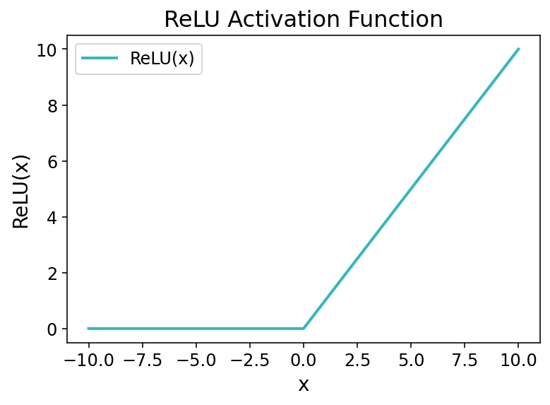
In the graph above, you’ll notice the sharp bend that occurs when x = 0, where the function transitions from zero to a linear increase for positive values. This change is exactly what allows your deep learning model to learn non-linear patterns, allowing it to learn complex relationships in our data.

The ReLU function can be defined as this:

# Defining the ReLU Function in Python
def relu(x):
    return max(0, x)

Our function accepts a single input, x and returns the maximum of either 0 or the value itself. This means that the ReLU function introduces non-linearity into our network by letting positive values pass through it unaffected while turning all negative values into zeros.

Let’s now dive into understanding the many benefits that the ReLU function provides for deep learning projects.

Understanding Why ReLU is Preferred for Deep Learning

Choosing the right activation function for deep learning projects is a critical decision to make. Over time, the Rectified Linear Unit (or ReLU) function emerged as one of the preferred choices in many neural network architectures.

In this section, we’ll explore why the ReLU function is a preferred function for many deep-learning projects.

Simplicity and Computational Efficiency

One of the main advantages of the ReLU function is its sheer simplicity. The function involves very little computation, making it computationally efficient compared to other, more complex functions like the sigmoid activation function.

This allows your models to train faster, which can be a huge consideration when working with complex models and large datasets.

Addressing the Vanishing Gradient Problem

The vanishing gradient problem is a common struggle with deep learning problems. This occurs when activation functions such as the sigmoid of the hyperbolic tangent create very small gradients for extreme values, which leads to slow convergence.

The ReLU activation function helps mitigate the vanishing gradient problem by providing a constant gradient for positive input values. When the input is positive, the gradient is simply 1, which means that the weights can easily be updated.

This property allows your models to train much more effectively, which can be essential for solving complex tasks.

Sparsity and Neural Efficiency

The ReLU function encourages sparsity in neural networks by zeroing out negative values, meaning that those neurons become inactive. This sparsity can lead to several advantages, such as memory efficiency since they require less memory to store.

Similarly, the neural efficiency of sparsity can lead to better generalization as the network focuses more on the relevant features and less on the ones that impact learning more.

Intuitive Behavior in Deep Learning

One of the most difficult challenges to overcome in deep learning is fostering intuition. Because the ReLU function is incredibly simple, it allows your model to become a little less complex. It mimics how human neurons work, where they activate when a certain threshold is crossed.

Because of this, it makes ReLU an important function when developing models that are meant to teach beginners or researchers who want to better understand how neural networks work.

Practical Implementation of the ReLU Activation Function in Python

So far, you have learned a lot about the rectified linear unit (ReLU) activation function and the important role it plays in deep learning. Let’s now dive a little further into how we can practically implement the function using Python and NumPy. We’ll walk through how to define the function and demonstrate how to use it on an array of data.

Let’s take a look at how we can define the ReLU activation function with NumPy:

# Defining ReLU with NumPy
import numpy as np

def relu(x):
    return np.maximum(0, x)

Similar to our pure Python function from earlier in the tutorial, the NumPy implementation uses a maximum() function to get the larger of either the value or 0. Because NumPy functions can work element-wise, this means we can pass in an entire array of values, rather than one value by itself.

Let’s see how we can use this function in practice:

# Using the ReLU Function
input_data = np.array([-2, -1, 0, 1, 2])
output_data = relu(input_data)
print("Input Data:", input_data)
print("Output Data (ReLU-transformed):", output_data)

# Returns:
# Input Data: [-2 -1  0  1  2]
# Output Data (ReLU-transformed): [0 0 0 1 2]

In the code block above, we first defined a NumPy array containing five numbers, some of which are positive and some are negative. We then passed this array into our newly-defined function. By printing out the input and output, we can see how the ReLU function transformed our original array.

In practice, you’ll often turn to a deep-learning function to implement the ReLU function – let’s explore how to implement the function in PyTorch.

Implementing the ReLU Activation Function in PyTorch

PyTorch is an immensely popular deep-learning library that provides tools for building and training neural networks efficiently. In the previous section, we explored how to implement the ReLU activation function in Python using NumPy. In this section, we’ll explore how to use the PyTorch library to implement and use the ReLU function.

PyTorch implements the rectified linear unit function (ReLU) using the nn module. Let’s see how we can create the function:

# Using PyTorch to Implement the ReLU Activation Function
import torch.nn as nn
relu = nn.ReLU()

In the code block above, we first imported the nn module using the conventional alias nn. We then defined a function object by instantiating the nn.ReLU class. We can now use the function by passing in values – let’s give that a shot:

# Using the ReLU Function in PyTorch
import torch
import torch.nn as nn

relu = nn.ReLU()
values = torch.tensor([-2, -1, 0, 1, 2])
transformed_values = relu(values)

print(transformed_values)

# Returns: tensor([0, 0, 0, 1, 2])

Let’s break down what we did in the code block above:

1. We imported both the torch library and the nn module
2. We then instantiated the function like we did before
3. Then, we created a PyTorch tensor containing values from -2 through +2
4. We then passed this tensor into the relu function object and printed the result

We can see that the values have been correctly transformed, changing all negative values to zero and keeping all positive values the same.

Commonly, you’ll want to implement the ReLU function as part of a neural network. Let’s see how we can build a simple neural network class to see how we can use the activation function in PyTorch:

# Implementing a Neural Network with ReLU in PyTorch
import torch
import torch.nn as nn
import torch.optim as optim

class SimpleNN(nn.Module):
    def __init__(self):
        super(SimpleNN, self).__init__()
        self.fc1 = nn.Linear(10, 5)
        self.relu = nn.ReLU()

    def forward(self, x):
        x = self.fc1(x)
        x = self.relu(x)
        return x

# Create an instance of the neural network
model = SimpleNN()

# Input data (as a PyTorch tensor)
input_data = torch.randn(1, 10) 

# Forward pass through the network
output_data = model(input_data)

In the code block above, we implemented a linear neural network and included the ReLU activation function inside it. We then instantiated the class and passed in a sample tensor. Let’s take a look at how we can explore these values:

print("Input Data:\n", input_data)
print("\nOutput Data (ReLU-transformed):\n", output_data)

# Returns:
# Input Data:
#  tensor([-5., -4., -3., -2., -1.,  0.,  1.,  2.,  3.,  4.])

# Output Data (ReLU-transformed):
#  tensor([0.3123, 0.4315, 2.4146, 0.0000, 0.0000, 0.0000, 2.2900, 0.0000, 2.6510,
#         0.0000], grad_fn=<ReluBackward0>)

In the code block above, we can see how passing a tensor of data through both a linear layer and then activating it using the ReLU function affects the data.

Now that you have learned how to implement the function in both NumPy and PyTorch, let’s explore a little bit more of the theory of the ReLU function, by learning how the function addresses the vanishing gradient problem.

Understanding How ReLU Addresses the Vanishing Gradient Problem

The vanishing gradient problem is a long-standing challenge faced by many neural networks. The vanishing gradient problem occurs while training neural networks, especially when using gradient-based optimization techniques. It occurs when the gradients of a loss function with respect to the model’s parameters become exceeding small as they are backpropagated through the network.

This is a common problem when using functions such as the sigmoid of Tanh activation functions. These functions are known to produce small gradients, especially for values far away from zero. This results in shrinking gradients, especially as networks get deeper and deeper. At some point, these weight updates become negligible, which impedes the training process and results in slow convergence or stagnation.

The behavior of ReLU’s gradients is different, however. ReLU provides a constant gradient of 1 for all positive values. This means that through backpropagation, gradients retain their magnitude and facilitate more effective weight updates. Similarly, for negative input values, ReLU provides a gradient of 0, which means that all negative gradients are simply ignored.

Put simply, the gradient behavior of ReLU addresses the vanishing gradient problem in two ways:

1. Gradients are not exponentially small: ReLU’s gradients are either 1 (for positive inputs) or 0 (for negative inputs), ensuring that gradients don’t vanish to the same extent.
2. Efficient propagation of gradients: The consistent gradient of 1 for positive values allows gradients to flow efficiently during backpropagation. This enables the network to adjust the weights more effectively, speeding up the convergence process.

However, the ReLU function can suffer from the dying ReLU problem where neurons in a network get stuck in an inactive state and never recover during training. Because of this, variations have been developed to address these problems. Let’s explore these in the next section.

Common Variations of the ReLU Activation Function

This tutorial has shown how valuable the ReLU function can be for deep learning. However, there are a few variations to the rectified linear unit function that can address certain challenges and help in specific cases. In this section, we’ll explore some of the common ReLU variations and discuss when you may want to use them.

Let’s take a look at what these variations look like:

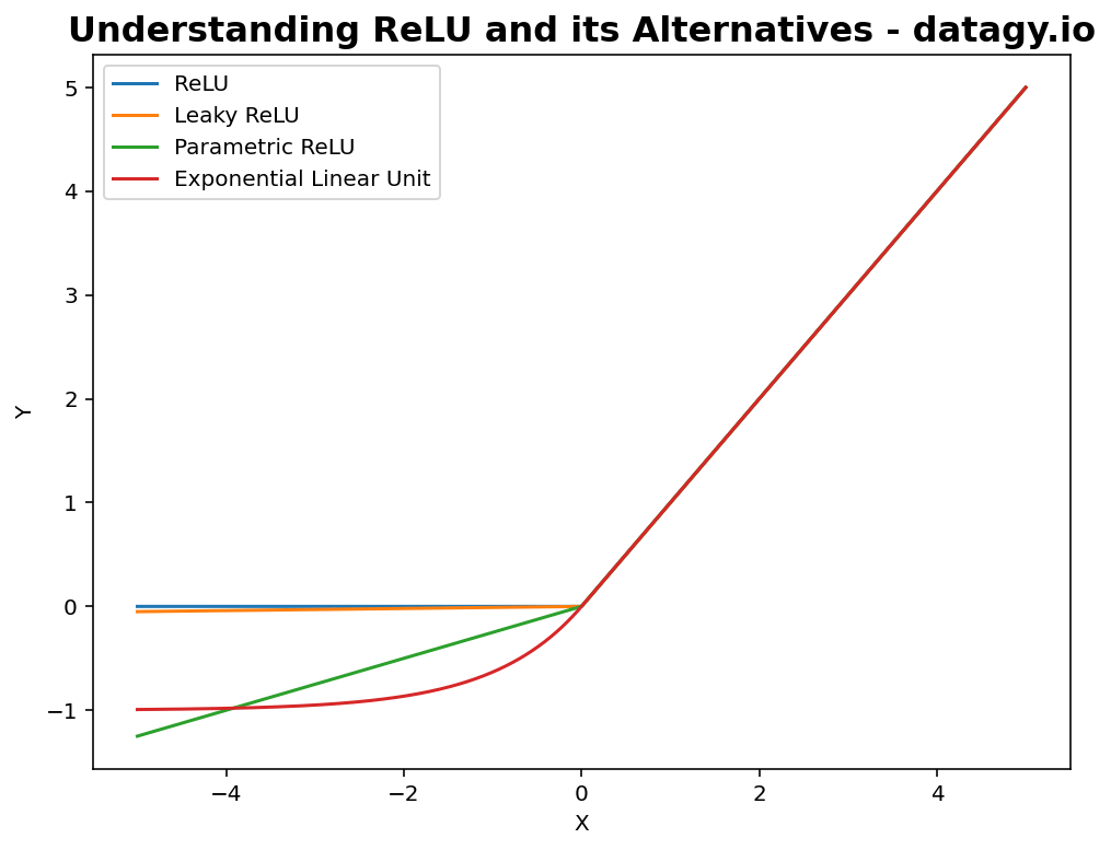
Now that you have a visual understanding of what these alternatives look like, let’s dive into each of them in detail.

Understanding the Leaky ReLU Function

The Leaky ReLU function is used to address the dying ReLU problem, where neurons can become inactive and never reactivate during training processes. It does this by introducing a small, non-zero gradient for negative inputs, which allows some information to flow through backpropagation, even when the input is negative.

Let’s take a look at the mathematical definition of the Leaky ReLU function:

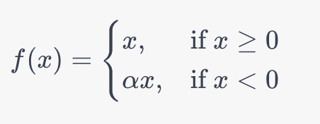
In the formula above, α introduces a small positive constant (typically, in the range of 0.01 and 0.3). This ensures that the neurons never become inactive, which allows the function to avoid the dying ReLU problem.

Understanding the Parametric ReLU (PReLU) Function

The Parametric ReLU function extends on the Leaky ReLU by introducing α as a parameter that is learned during the training process, rather than being a fixed constant. This enables the neural network to adapt the slope of the negative side of the activation function, based on the specific problem the function is meant to solve.

Let’s take a look at the mathematical function behind the Parametric ReLU function:

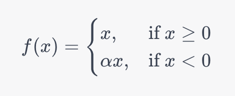
This function is exceptionally useful when you have a large dataset with wildly varied characteristics. This is because the function can learn the optimal slope for the negative input values, addressing issues that can arise eve in the Leaky ReLU function.

Understanding the Exponential Linear Unit (ELU) Function

The Exponential Linear Unit (ELU) Function looks to combine the advantages of the ReLU and the Leaky ReLU function while adding some unique properties. Let’s take a look at the ELU function definition and explore what makes it unique:

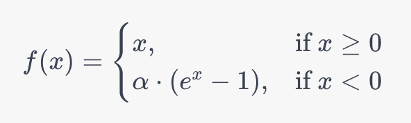
While the ELU retains the functionality of ReLU for positive numbers, the behavior varies for negative values. On the negative side of the function, an exponential curve is used to handle negative inputs more smoothly than the ReLU or Leaky ReLU. This has been shown in practice to learn faster convergence and improved generalization.

When to Use Variations on the ReLU Function

With all of these variations of the regular ReLU function, it can seem like a daunting task to understand when to use which function. The table below breaks down the most common use cases for each of the ReLU function variations:

Function	Use Case
ReLU (standard)	The standard ReLU is used when you want a simple and computationally efficient activation function are aren’t worried about the dying ReLU problem.
Leaky ReLU	The Leaky ReLU should be used when you want to mitigate the dying ReLU problem and when you want to have a small, fixed gradient for negative inputs.
Parametric ReLU (PReLU)	The PReLU is best for when you want the network to learn the optimal slope for negative inputs, which can be useful for varying data distributions.
Exponential Linear Unit (ELU)	The ELU is best used when you want a smooth activation function that handles negative inputs gracefully, which can lead to faster training and better generalization.

In this section, we explored the variation of the ReLU activation function and what the best use cases for each function are.

Handling Common Issues with the ReLU Activation Function

While the Rectified Linear Unit (ReLU) and its variations provide many advantages over other activation functions, they also come with some challenges of their own. In this section, we’ll explore what some of the most common challenges are and how to address them.

Addressing the Exploding Gradient Problem When Using ReLU

While the ReLU function alternatives address the dying ReLU problem, it can lead to another problem: the exploding gradient problem. This problem occurs when gradients become too large during backpropagation, causing weight updates to become too large and destabilize training. In order to address this problem, you can implement the following solutions:

• Gradient clipping: By scaling down gradients if they exceed a certain threshold, you can prevent gradients from becoming excessively large.
• Learning Rate Scheduling: In order to help stabilize weights, you can reduce the learning rate as training progresses.

Addressing Learning Rate Sensitivity When Using ReLU

Choosing the appropriate learning rate is crucial for training stable and effective models. This is especially true when using the ReLU activation function due to its sensitivity to learning rates. This is because ReLU has either gradients of 0 or 1, making it very sensitive to the learning rate. You can address this problem by implementing the following solutions:

• Learning Rate Scheduling: This technique gradually reduces the learning rate during training, starting with a relatively large rate for faster convergence. Common learning rate schedules include step decay or exponential decay.
• Monitoring Loss and Gradient Magnitudes: By plotting the loss curve and monitoring gradient statistics, you can identify if the learning rate is too high or too low. This allows you to easily use tools such as early stopping to prevent overfitting.

In this section, we discussed some of the challenges that are associated with the ReLU function and how to address these challenges.

Conclusion

In this guide, we explored the rectified linear unit, or ReLU, in-depth. We first learned how the function works and what makes it unique from other activation functions. We also explored how the function can be implemented in Python using NumPy as well as PyTorch. From there, we explored some of the benefits and drawbacks of the function. Finally, we also explored what some of the alternatives to the function are and what benefits they bring.

To learn more about how to implement ReLU in PyTorch, check out the official documentation.