
In this post, we’ll learn how to use VLOOKUP in Excel! VLOOKUP is an Excel function that can look up data in one Excel table and return it in another. The function runs similarly to the HLOOKUP function, but searches for data vertically (hence the “v”). VLOOKUP in Excel lets you return matches for specific data pieces that may otherwise take a lot of manual work to find. Let’s take a look at how the function can be used properly.
Table of Contents
Understanding the VLOOKUP Function
The function looks like this:
=VLOOKUP(lookup_value, table_array, col_index_num, [range_lookup])The first three parameters are required, but the fourth is optional and will default to TRUE if left alone. Let’s explore these a bit in more detail:
- Lookup Value: the value that you’re asking Excel to search for in the your lookup table. The value can be a number of different data types:
- Number: simply enter any number (e.g., VLOOKUP(40, table_array, col_index_num, [range_lookup])
- Text: search for any string of text by including double quotes around the search criteria (e.g., VLOOKUP(“dog”, table_array, col_index_num, [range_lookup])
- Cell Reference: enter a cell reference as the parameter (e.g., VLOOKUP(A1, table_array, col_index_num, [range_lookup])
- Table Array: the array (or table) that you’re asking Excel to search in for your other data
- Excel will only search in the first column for the lookup value of the array you’re providing.
- Column Index Number (col_index_num): the column from which you’re asking Excel to return data from
- The left-most column in your array is column 1, and are incremented by 1 as you move right.
- Range Lookup (optional): accepts two values (FALSE and TRUE) and determines whether you want to use an exact or approximate match
- While the parameter is optional, how you use it has significant impact on your results and we’ll explore that in more detail below
How to Use VLOOKUP in Excel
Let’s take a look at an example of how to use VLOOKUP. Similar to our Getting Started with SQL guide, we’ll use two tables that relate to an online store.
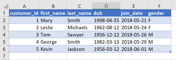
- Our first table will exist on a sheet called Clients and we’ll assume the table has been named clients. The table covers the range clients!$A$1:$F$6
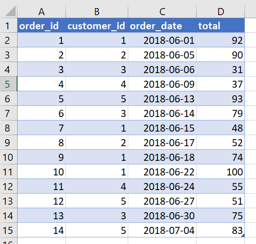
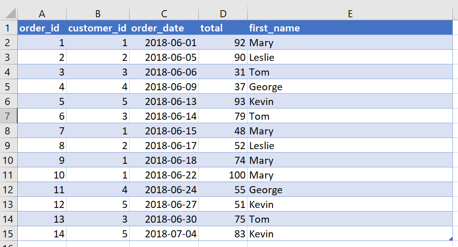
- Our second table will exist on a sheet called Orders and we’ll assume the table is called orders. The table covers the range orders!$A$1:$D$15
Our table clients looks like this:
Our table orders looks like this:
Say we wanted to construct a lookup that return’s the customer’s first name based on their order number and looks a little like this:
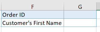
Our goal is to be able to enter an order_id and return the customer’s first name.
Forming the VLOOKUP Function
To start, let’s begin writing out the VLOOKUP function, which we’d enter into cell G2
=VLOOKUP(G1, clients!$A$1:$F$6, 2, FALSE)Let’s explore this in a bit of detail:
| Parameter | Example | Details |
| Lookup Value | G1 | Into G1, we’ll enter any client_id that exists in the clients table. As we change this value, the returned first name will also update. |
| Table Array | clients!$A$1:$F$6 | Selects the entire range of the table. Note: the lookup will only work correctly if the lookup value is in the left-most column. |
| Column Index Number | 2 | Tells Excel to return the value in the 2nd column, adjacent to the looked up value. |
| Range Lookup | FALSE | Tells Excel to return an exact match only. (we’ll explore this more below) |
As we change the value we enter into G1, the returned value will update based on the client’s first name. If the client_id doesn’t exist in the clients table, Excel will return a #N/A error (provided the FALSE range lookup value is retained).
Applying VLOOKUP to an Entire Column
Similarly to the example above, we can also apply VLOOKUP in Excel to an entire column. For example, if we wanted to return the first name of the client for each order, we could enter the function into a column as part of the order’s table:
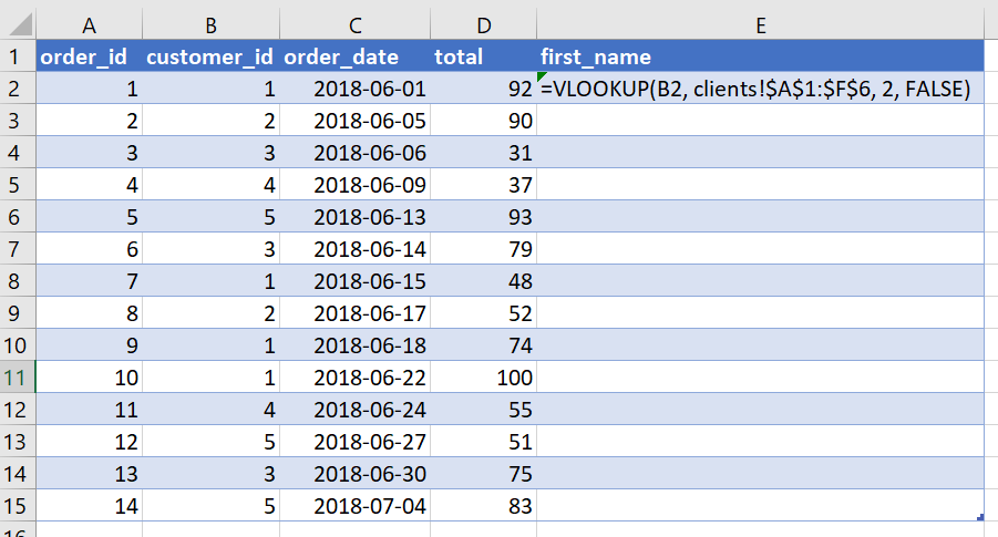
When we enter this function, we get the following result:
Do you use TRUE or FALSE for a VLOOKUP Range Lookup?
Using TRUE (VLOOKUP’s default value) or FALSE will have some significant impacts on the result that your function will return. Let’s take a quick look:
- If you’re wanting on exact matches
(e.g., looking up names), you’ll want to use FALSE
- If the looked up value doesn’t exist, an #N/A error will be returned
- If you’re wanting approximate matches, use TRUE
How do Approximate/Fuzzy Matches work in VLOOKUP?
An approximate match does a number of things:
- It searches for an exact match. If an exact match is not found,
- It looks for the closest maximum value
that is less than the value searched for.
- For this to work, the lookup range must be in ascending order.
Some Important Notes on VLOOKUP
VLOOKUP only returns the first match: if the lookup value exists in your range more than once, only the first value is returned.
VLOOKUP is case sensitive: searching for “Mary” or “MARY” will yield different results.
VLOOKUP will work with named ranges: in our example above, since we had named the ranges the table sit on (clients and orders), we could have referenced those ranges by name rather than by their cell arrays.
Additional Resources:
- Create Dropdown List in Excel
- Setting up a Personal Macro Workbook in Excel (and some sample macros!)
- You can learn more about the function by checking the official documentation.